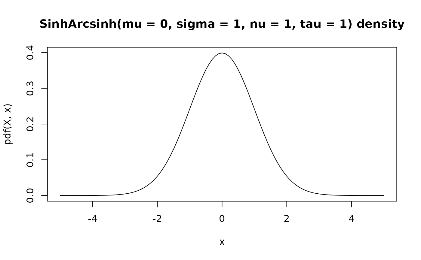
The Sinh-Arcsinh (SHASH) distribution is a four-parameter distribution with support on the real space that generalizes the Normal distribution by separately controlling location, scale, skewness, and tail-heaviness. It can produce a wide range of shapes, including symmetric and asymmetric forms and both heavier and lighter tails, making it useful for modeling real-valued data with non-normal behavior. Using \(\nu = 1\) and \(\tau = 1\) results in a standard normal distribution.
Details
We recommend reading this documentation on https://zeileis.github.io/distributions3/, where the math will render with additional detail and much greater clarity.
In the following, let \(X\) be a Sinh-Arcsinh random variable with mean
mu = \(\mu\), sigma = \(\sigma\), nu = \(\nu\), and
tau = \(\tau\).
Support: \(R\), the set of all real numbers
Probability density function (p.d.f):
$$ f(t) = \frac{1}{\sigma \sqrt{1 + z^2}} \cdot \frac{1}{2}\left(\tau e^{\tau w} + \nu e^{-\nu w}\right) \cdot \phi\left( \frac{1}{2}\left(e^{\tau w} - e^{-\nu w}\right) \right) $$
$$ \text{where } z = \frac{t - \mu}{\sigma}, ~w = \operatorname{asinh}(z), ~\text{and } \phi() \text{ is the standard normal PDF.} $$
Cumulative distribution function (c.d.f):
$$ F(t) = \Phi\left( H\left(\operatorname{asinh}\left(\frac{t - \mu}{\sigma}\right)\right) \right) $$
$$ \text{where } H(w) = \frac{1}{2}\left(e^{\tau w} - e^{-\nu w}\right), ~\text{and } \Phi() \text{ the standard normal CDF.} $$
References
Jones MC, Pewsey A (2009). “Sinh-Arcsinh Distributions”, Journal of Statistical Software, 96(4), 761–780. doi:10.1093/biomet/asp053
See also
Other continuous distributions:
Beta(),
Cauchy(),
ChiSquare(),
Erlang(),
Exponential(),
FisherF(),
Frechet(),
GEV(),
GP(),
Gamma(),
Gumbel(),
LogNormal(),
Logistic(),
Normal(),
RevWeibull(),
StudentsT(),
Tukey(),
Uniform(),
Weibull()
Examples
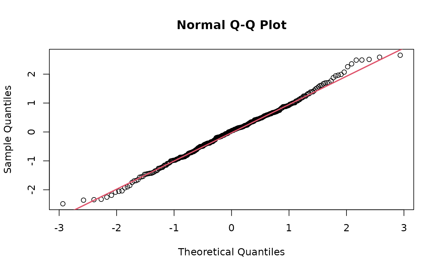
## SinhArcsinh() by default uses nu = 1, tau = 1 which
## results in the standard normal distribution
set.seed(6020)
X <- SinhArcsinh() # Uses mu = 1, sigma = 0, nu = 1, tau = 1)
x <- random(X, 300)
qqnorm(x); qqline(x, col = 2, lwd = 2)
 curve(pdf(X, x), xlim = c(-5, 5), main = paste(X, "density"))
 ## Calculation of central moments is based on numeric integration,
## thus not being identical to the standard normal distribution
c(mean = mean(x), sd = sd(x))
#> mean sd
#> 0.001386471 0.999227517
## Skewed Sinh-Arcsinh distribution
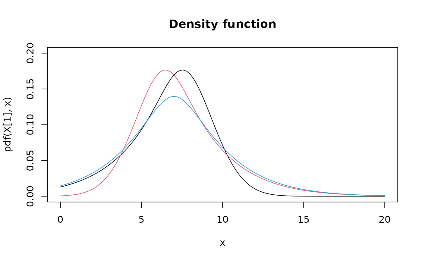
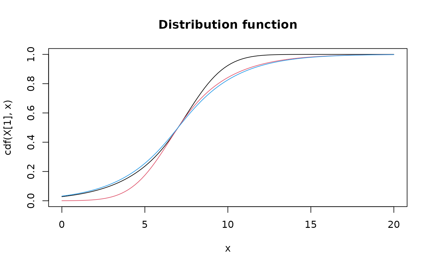
X <- SinhArcsinh(mu = 7, sigma = 2, nu = c(0.7, 1, 0.7), tau = c(1, 0.7, 0.7))
as.matrix(X)
#> mu sigma nu tau
#> [1,] 7 2 0.7 1.0
#> [2,] 7 2 1.0 0.7
#> [3,] 7 2 0.7 0.7
## Visualization of density functions using different parameters for nu/tau
curve(pdf(X[1], x), xlim = c(0, 20), ylim = c(0, 0.2), main = "Density function")
curve(pdf(X[2], x), xlim = c(0, 20), col = 2, add = TRUE)
curve(pdf(X[3], x), xlim = c(0, 20), col = 4, add = TRUE)
## Calculation of central moments is based on numeric integration,
## thus not being identical to the standard normal distribution
c(mean = mean(x), sd = sd(x))
#> mean sd
#> 0.001386471 0.999227517
## Skewed Sinh-Arcsinh distribution
X <- SinhArcsinh(mu = 7, sigma = 2, nu = c(0.7, 1, 0.7), tau = c(1, 0.7, 0.7))
as.matrix(X)
#> mu sigma nu tau
#> [1,] 7 2 0.7 1.0
#> [2,] 7 2 1.0 0.7
#> [3,] 7 2 0.7 0.7
## Visualization of density functions using different parameters for nu/tau
curve(pdf(X[1], x), xlim = c(0, 20), ylim = c(0, 0.2), main = "Density function")
curve(pdf(X[2], x), xlim = c(0, 20), col = 2, add = TRUE)
curve(pdf(X[3], x), xlim = c(0, 20), col = 4, add = TRUE)
 ## Visualization of distribution function using different parameters for nu/tau
curve(cdf(X[1], x), xlim = c(0, 20), ylim = 0:1, main = "Distribution function")
curve(cdf(X[2], x), xlim = c(0, 20), col = 2, add = TRUE)
curve(cdf(X[3], x), xlim = c(0, 20), col = 4, add = TRUE)
## Visualization of distribution function using different parameters for nu/tau
curve(cdf(X[1], x), xlim = c(0, 20), ylim = 0:1, main = "Distribution function")
curve(cdf(X[2], x), xlim = c(0, 20), col = 2, add = TRUE)
curve(cdf(X[3], x), xlim = c(0, 20), col = 4, add = TRUE)
 ## Central moments
mean(X)
#> [1] 6.579299 7.420701 7.000000
variance(X)
#> [1] 7.988051 7.988051 13.222747
skewness(X)
#> [1] -0.9964539 0.9964539 0.0000000
kurtosis(X)
#> [1] 1.986356 1.986356 1.381735
## Drawing random values
random(X, 10)
#> r_1 r_2 r_3 r_4 r_5 r_6 r_7 r_8
#> [1,] 1.620320 5.822669 4.726385 4.9665369 7.328488 6.761931 9.695683 7.278853
#> [2,] 9.948123 7.289761 9.029897 8.0250984 10.712057 6.556041 8.718336 6.313155
#> [3,] 3.137213 6.323366 7.701549 -0.6735327 7.391669 7.226570 3.741789 5.985342
#> r_9 r_10
#> [1,] 6.251743 4.153261
#> [2,] 8.554793 2.064297
#> [3,] 4.288999 7.089715
pdf(X, 2)
#> [1] 0.02952215 0.01025629 0.03267175
log_pdf(X, 2)
#> [1] -3.522614 -4.579864 -3.421245
cdf(X, 4)
#> [1] 0.15803712 0.07568062 0.17430273
quantile(X, 0.7)
#> [1] 8.152092 8.385512 8.563814
# note that the cdf() and quantile() functions are inverses
X <- SinhArcsinh(mu = 3, sigma = 2, nu = 0.9, tau = 1.2)
cdf(X, quantile(X, 0.7))
#> [1] 0.7
quantile(X, cdf(X, 7))
#> [1] 7
## Central moments
mean(X)
#> [1] 6.579299 7.420701 7.000000
variance(X)
#> [1] 7.988051 7.988051 13.222747
skewness(X)
#> [1] -0.9964539 0.9964539 0.0000000
kurtosis(X)
#> [1] 1.986356 1.986356 1.381735
## Drawing random values
random(X, 10)
#> r_1 r_2 r_3 r_4 r_5 r_6 r_7 r_8
#> [1,] 1.620320 5.822669 4.726385 4.9665369 7.328488 6.761931 9.695683 7.278853
#> [2,] 9.948123 7.289761 9.029897 8.0250984 10.712057 6.556041 8.718336 6.313155
#> [3,] 3.137213 6.323366 7.701549 -0.6735327 7.391669 7.226570 3.741789 5.985342
#> r_9 r_10
#> [1,] 6.251743 4.153261
#> [2,] 8.554793 2.064297
#> [3,] 4.288999 7.089715
pdf(X, 2)
#> [1] 0.02952215 0.01025629 0.03267175
log_pdf(X, 2)
#> [1] -3.522614 -4.579864 -3.421245
cdf(X, 4)
#> [1] 0.15803712 0.07568062 0.17430273
quantile(X, 0.7)
#> [1] 8.152092 8.385512 8.563814
# note that the cdf() and quantile() functions are inverses
X <- SinhArcsinh(mu = 3, sigma = 2, nu = 0.9, tau = 1.2)
cdf(X, quantile(X, 0.7))
#> [1] 0.7
quantile(X, cdf(X, 7))
#> [1] 7