Density (point mass), distribution, quantile function, as well as a random generation for the Empirical distribution.
Usage
dempirical(x, y, log = FALSE, na.rm = TRUE, method = NULL, ...)

pempirical(q, y, lower.tail = TRUE, log.p = FALSE, na.rm = TRUE)

qempirical(
  p,
  y,
  lower.tail = TRUE,
  log.p = FALSE,
  na.rm = TRUE,
  type = 1L,
  ...
)

rempirical(n, y, na.rm = TRUE)
Arguments
- x
Vector of finite quantiles.
- y
Vector of observations of the empirical distribution with two or more non-missing finite values.
- log, log.p
logical. Indicates whether probabilities p are given as log(p) (both default to
FALSE).- na.rm
logical indicating whether missing values (
NA) are stripped before computation, defaults toTRUE.- method
NULLor one of"hist"or"density". IfNULL,yis considered a random variable from a discrete empirical distribution. Method"hist"and"density"approximate a 'continuous' distribution based on the empirical sampley.- ...
Allows to forward arguments to
hist,density()andapply/sapplywhen callingdempirical()or samplequantilefunction when callingqempirical(). Else currently unused.- q
vector of quantiles.
- lower.tail
logical indicating whether probabilities are \(P[X \le x]\) (lower tail) or \(P[X > x]\) (upper tail).
- p
numeric vector of probabilities (
[0, 1]).- type
integer, forwarded to
quantile. Defaults totype = 1L.- n
number of observations. If
length(n) > 1, the length is taken to be the number required.
Details
All functions follow the usual conventions of d/p/q/r functions in base R. In
particular, all four functions for the Empirical distribution call
the corresponding *empirical functions.
See also
Other Empirical distribution:
Empirical(),
cdf.Empirical(),
pdf.Empirical(),
quantile.Empirical(),
random.Empirical(),
support.Empirical()
Examples
## Drawing two random empirical sample Y from the LogNormal distribution
## rounded to closest 0.5 (discrete)
set.seed(6020)
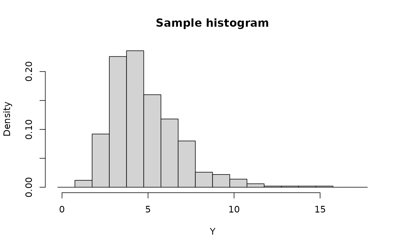
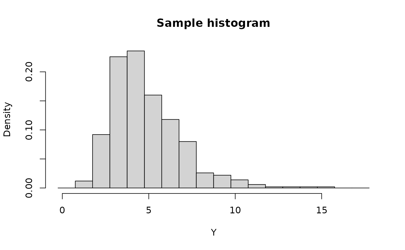
Y <- rlnorm(500L, meanlog = 1.5, sdlog = log(1.5))
Y <- round(Y * 2) / 2
bk <- seq(-0.25, 18.25, by = 1L)
hist(Y, freq = FALSE, breaks = bk, main = "Sample histogram")
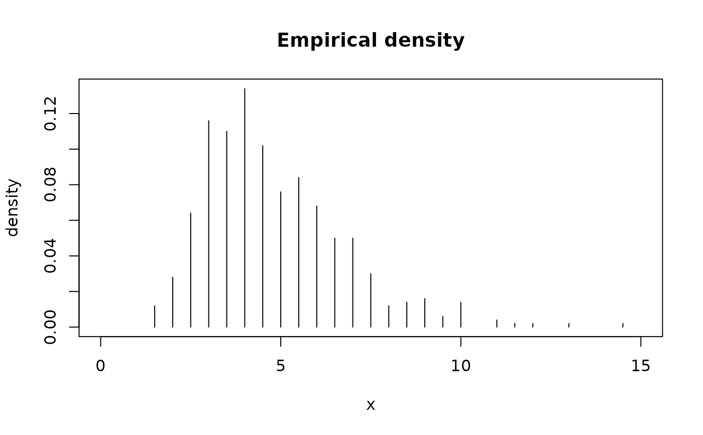
 x <- seq(0, 15, by = 0.5) # Quantiles
density <- dempirical(x, Y)
plot(density ~ x, type = "h", main = "Empirical density")
x <- seq(0, 15, by = 0.5) # Quantiles
density <- dempirical(x, Y)
plot(density ~ x, type = "h", main = "Empirical density")
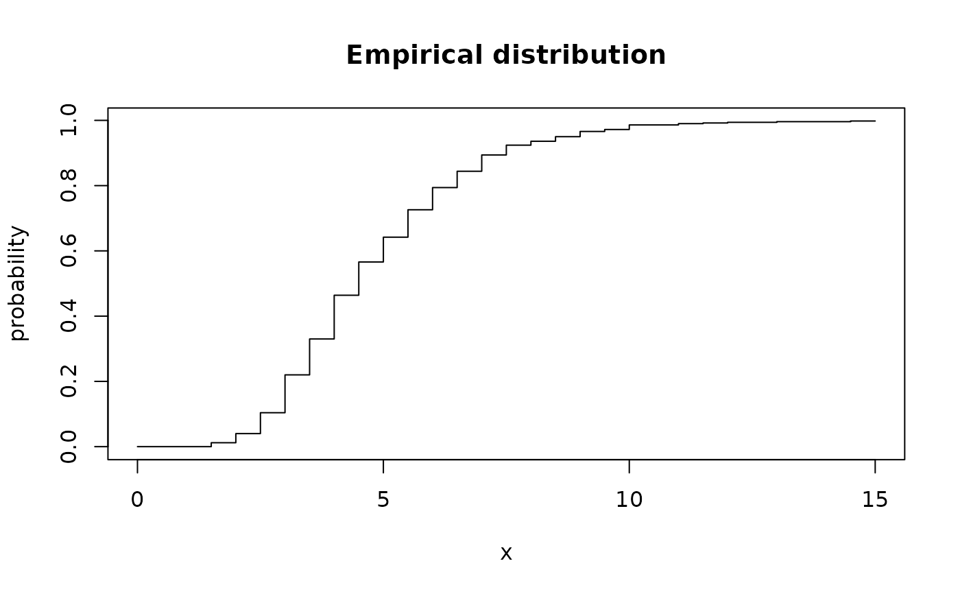
 probability <- pempirical(x, Y)
plot(probability ~ x, type = "s", main = "Empirical distribution")
probability <- pempirical(x, Y)
plot(probability ~ x, type = "s", main = "Empirical distribution")
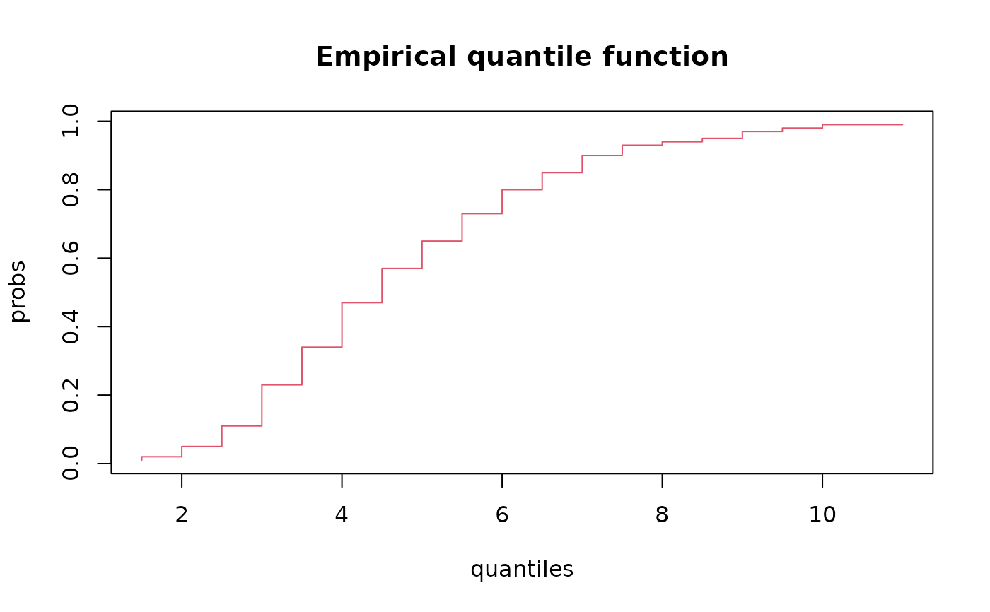
 probs <- seq(0.01, 0.99, by = 0.01)
quantiles <- qempirical(probs, Y)
plot(probs ~ quantiles, type = "S", col = 2,
main = "Empirical quantile function")
probs <- seq(0.01, 0.99, by = 0.01)
quantiles <- qempirical(probs, Y)
plot(probs ~ quantiles, type = "S", col = 2,
main = "Empirical quantile function")
 ## Drawing random numbers (sampling with replacement)
set.seed(6020)
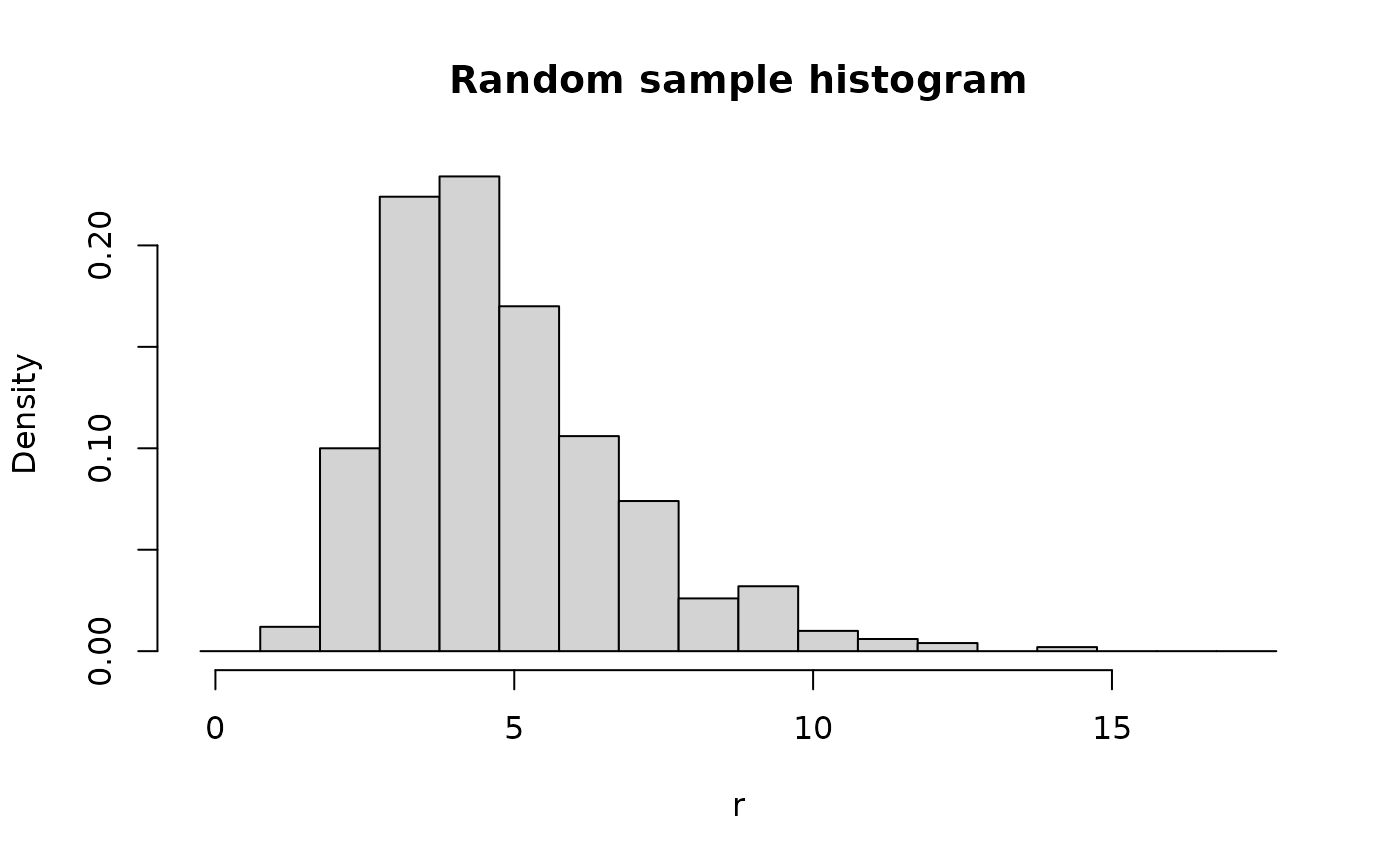
r <- rempirical(500L, Y)
hist(Y, freq = FALSE, breaks = bk, main = "Sample histogram")
## Drawing random numbers (sampling with replacement)
set.seed(6020)
r <- rempirical(500L, Y)
hist(Y, freq = FALSE, breaks = bk, main = "Sample histogram")
 hist(r, freq = FALSE, breaks = bk, main = "Random sample histogram")