Methods for numerically approximating distribution functions
Source:R/distribution.R
pdf.distribution.RdS3 methods for distribution objects used if certain (analytic) distribution functions are not available. Allows to use all distributions3 methods even if there are no dedicated methods for a certain distribution. See section 'Details' for more information.
Usage
# S3 method for class 'distribution'
pdf(
  d,
  x,
  drop = TRUE,
  elementwise = NULL,
  log = FALSE,
  applyfun = NULL,
  cores = NULL,
  ...
)

# S3 method for class 'distribution'
log_pdf(d, x, ...)

# S3 method for class 'distribution'
quantile(
  x,
  probs,
  drop = TRUE,
  elementwise = NULL,
  lower = -1/sqrt(.Machine$double.eps),
  upper = +1/sqrt(.Machine$double.eps),
  tol = .Machine$double.eps^0.5,
  maxit = 1000,
  ...
)

# S3 method for class 'distribution'
cdf(d, x, drop = TRUE, elementwise = NULL, lower.tail = TRUE, ...)
Arguments
- d
An object of class
distribution.- x
Either a numeric vector of probabilities to be evaluated (if
pdf()is called), or an object of classdistributionswhen calling thequantile()function.- drop
logical. Should the result be simplified to a vector if possible?
- elementwise
logical. Should each distribution (in
d/x) be evaluated at all elements inx(whenpdf()is called) orprobs(ifquantile()is called)? By default (ifelementwise = NULL) it is set toelementwise = TRUEif the lengths match, elseelementwiseis setFALSE.- log
logical. If
TRUE, probabilities are given aslog(p).- applyfun
An optional
lapply-style function with argumentsfunction(X, FUN, ...). It is used to compute the CRPS for each element ofy. The default is to use the basiclapplyfunction unless thecoresargument is specified (see below).- cores
NULLor positive integer. If set to an integer theapplyfunis set tomclapplywith the desired number ofcores, except on Windows whereparLapplywithmakeCluster(cores)is used.- ...
Currently ignored.
- probs
Numeric vector of probabilities with values in
[0,1].- lower, upper
numeric. Lower and upper end points for the interval to be searched, forwarded to
uniroot.- tol
numeric. Desired accuracy for
uniroot.- maxit
integer. Maximum number of iterations used when iteratively evaluating quantiles based on a pdf (discrete distributions only). If
maxitis reached before the quantile has been found, an error will be thrown.- lower.tail
logical. If
TRUE(default), probabilities are \(P[X \le x]\), else \(P[X \ge x]\).
Details
For distribution classes that do not (or not yet) provide all S3 methods for
the usual generic functions (pdf, cdf, quantile, random), a fallback
method for the general distribution class is provided. This fallback
method numerically approximates
the probability density function (PDF), cumulative distribution
function (CDF), quantile function, or random number generation,
provided that at least some of the methods are available (see below).
S3 methods for is_discrete and support are mandatory. Besides
these two (fairly simple) methods, the following methods are required.
Continuous distributions:
provide a
cdf.*method,or a
pdf.*andquantile.*method.
Discrete distributions:
provide a
pdf.*method,or a
cdf.*method.
Any additional S3 method provided on top of the minimal requirements will always be leveraged if available (i.e., the more dedicated/analytical methods provided the better).
Examples
## ------------- custom Normal distribution (MyNormal1) ---------------
## -------------------------- using cdf -------------------------------
## Constructor function for new 'MyNormal1' distribution
MyNormal1 <- function(mu, sigma) {
d <- data.frame(mu = mu, sigma = sigma)
class(d) <- c("MyNormal1", "distribution")
return(d)
}
## Additionally required S3 methods (borrowed from class Normal)
registerS3method("cdf", "MyNormal1",
getS3method("cdf", class = "Normal"))
registerS3method("is_discrete", "MyNormal1",
getS3method("is_discrete", class = "Normal"))
registerS3method("support", "MyNormal1",
getS3method("support", class = "Normal"))
## Constructing objects; three normal distributions with
## mean c(1, 2, 3) and standard deviation c(1, 2.5, 5).
## mn3: Based on MyNormal1 where only cdf, id_discrete, and support
## are defined.
## n3: Analytic solution (Normal()) with analytic functions
## for all distribution functions (pdf, cdf, quantile) as well as for
## the first four central moments (mean, variance, skewness, kurtosis)
mn3 <- MyNormal1(mu = 1:3, sigma = c(1, 2.5, 5))
n3 <- Normal(mu = 1:3, sigma = c(1, 2.5, 5))
## Class 'MyNormal1' knows the analytic cdf:
cdf(mn3, x = 2)
#> [1] 0.8413447 0.5000000 0.4207403
identical(cdf(mn3, x = 2), cdf(n3, x = 2))
#> [1] TRUE
## Calculating probability at x = 2
pdf(mn3, x = 2) ## Numeric approximation
#> [1] 0.24197072 0.15957691 0.07820854
pdf(n3, x = 2) ## Analytic solution
#> [1] 0.24197072 0.15957691 0.07820854
pdf(mn3, x = 2) - pdf(n3, x = 2) ## Pairwise differences/precision
#> [1] -2.982198e-12 -1.708411e-12 -9.030138e-13
## Calculating quantiles
probs <- c(0.0, 0.01, 0.25, 0.5, 0.75, 0.99, 1.0)
quantile(mn3, probs = probs) ## Numeric approximation
#> q_0 q_0.01 q_0.25 q_0.5 q_0.75 q_0.99 q_1
#> [1,] -Inf -1.326348 0.3255102 1 1.674490 3.326348 Inf
#> [2,] -Inf -3.815870 0.3137756 2 3.686224 7.815870 Inf
#> [3,] -Inf -8.631739 -0.3724488 3 6.372449 14.631739 Inf
quantile(n3, probs = probs) ## Analytic solution
#> q_0 q_0.01 q_0.25 q_0.5 q_0.75 q_0.99 q_1
#> [1,] -Inf -1.326348 0.3255102 1 1.674490 3.326348 Inf
#> [2,] -Inf -3.815870 0.3137756 2 3.686224 7.815870 Inf
#> [3,] -Inf -8.631739 -0.3724488 3 6.372449 14.631739 Inf
probs2 <- seq(0.01, 0.99, by = 0.01)
qmn3 <- quantile(mn3, probs = probs2) ## Numeric approximation
qn3 <- quantile(n3, probs = probs2) ## Analytic solution
range(qmn3 - qn3) ## Range of pairwise differences/precision
#> [1] -3.692192e-09 3.669803e-09
## Central moments
cbind(mean = mean(mn3), variance = variance(mn3),
skewness = skewness(mn3), kurtosis = kurtosis(mn3))
#> mean variance skewness kurtosis
#> [1,] 1 1.000463 -1.830206e-15 -2.568781e-07
#> [2,] 2 6.250463 3.383851e-10 -8.880798e-09
#> [3,] 3 24.926837 -1.034930e-12 -3.211273e-02
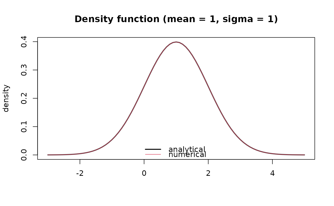
## Visual comparison: density
x <- seq(-3, 5, by = 0.1)
pmn3 <- pdf(mn3[1], x = x)
pn3 <- pdf(n3[1], x = x)
dpdf <- data.frame(x = x,
analytical = pdf(n3[1], x = x),
numerical = pdf(mn3[1], x = x))
matplot(dpdf[, 1], dpdf[, -1], type = "l", col = 1:2,
xlab = NA, ylab = "density", lty = 1, lwd = 2:1,
main = "Density function (mean = 1, sigma = 1)")
legend("bottom", legend = names(dpdf)[-1], bty = "n",
col = 1:2, lty = 1, lwd = 2:1)
 ## Visual comparison: quantiles
probs <- c(0.001, seq(0.01, 0.99, by = 0.01), 0.999)
dquantile <- data.frame(probs = probs,
analytical = quantile(n3[1], probs = probs),
numerical = quantile(mn3[1], probs = probs))
matplot(dquantile[, -1], dquantile[, 1], type = "l", col = 1:2,
xlab = NA, ylab = "probability", lty = 1, lwd = 2:1,
main = "Quantile function (mean = 1, sigma = 1)")
legend("bottom", legend = names(dquantile)[-1], bty = "n",
col = 1:2, lwd = 2:1)
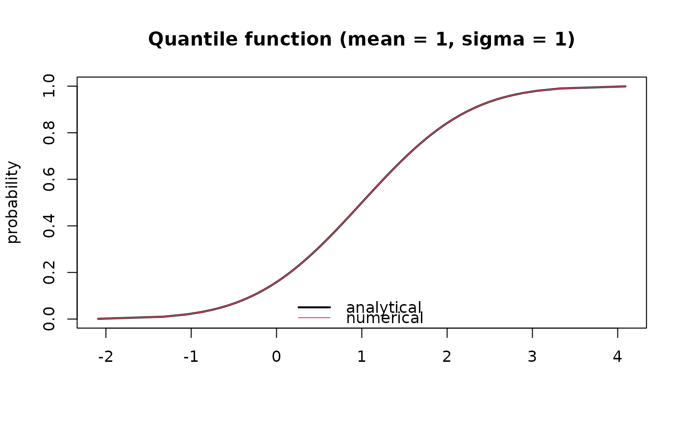
## Visual comparison: quantiles
probs <- c(0.001, seq(0.01, 0.99, by = 0.01), 0.999)
dquantile <- data.frame(probs = probs,
analytical = quantile(n3[1], probs = probs),
numerical = quantile(mn3[1], probs = probs))
matplot(dquantile[, -1], dquantile[, 1], type = "l", col = 1:2,
xlab = NA, ylab = "probability", lty = 1, lwd = 2:1,
main = "Quantile function (mean = 1, sigma = 1)")
legend("bottom", legend = names(dquantile)[-1], bty = "n",
col = 1:2, lwd = 2:1)
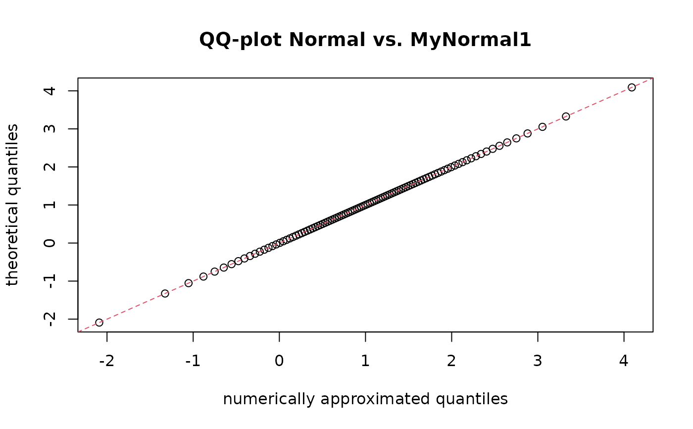
 ## Visual comparison: quantile-quantile plot
plot(dquantile[, "analytical"], dquantile[, "analytical"],
xlab = "numerically approximated quantiles",
ylab = "theoretical quantiles",
main = "QQ-plot Normal vs. MyNormal1")
abline(0, 1, col = 2, lty = 2)
## Visual comparison: quantile-quantile plot
plot(dquantile[, "analytical"], dquantile[, "analytical"],
xlab = "numerically approximated quantiles",
ylab = "theoretical quantiles",
main = "QQ-plot Normal vs. MyNormal1")
abline(0, 1, col = 2, lty = 2)
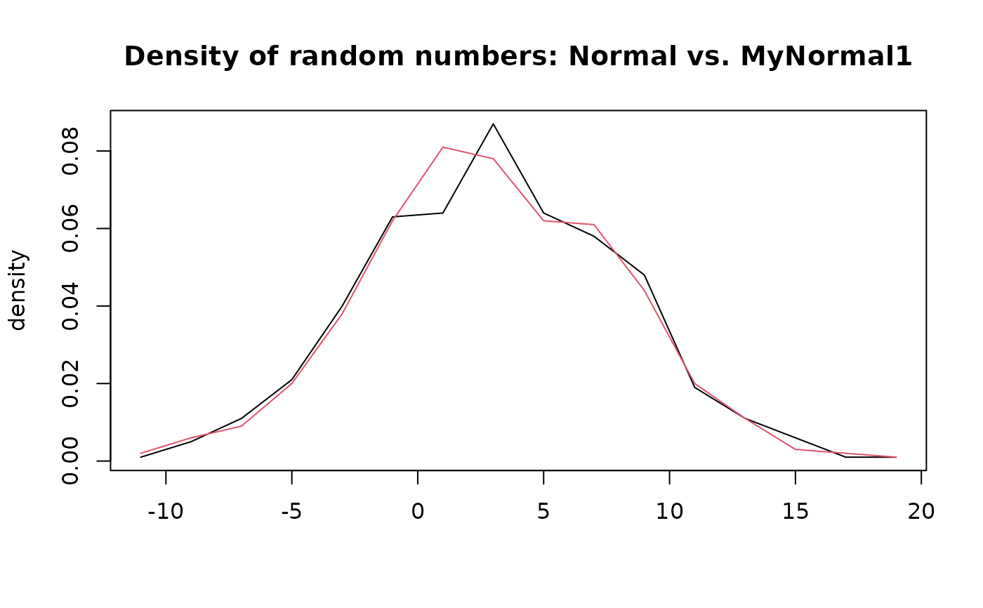
 ## Drawing random numbers (500 on third distribution)
set.seed(6020); rmn <- random(mn3[3], 500L)
set.seed(6020); rn <- random(n3[3], 500L)
hmn <- hist(rmn, breaks = 15L, plot = FALSE)
hn <- hist(rn, breaks = 15L, plot = FALSE)
plot(hmn$mids, hmn$density, type = "l",
xlab = NA, ylab = "density",
main = "Density of random numbers: Normal vs. MyNormal1")
lines(hn$mids, hn$density, col = 2)
## Drawing random numbers (500 on third distribution)
set.seed(6020); rmn <- random(mn3[3], 500L)
set.seed(6020); rn <- random(n3[3], 500L)
hmn <- hist(rmn, breaks = 15L, plot = FALSE)
hn <- hist(rn, breaks = 15L, plot = FALSE)
plot(hmn$mids, hmn$density, type = "l",
xlab = NA, ylab = "density",
main = "Density of random numbers: Normal vs. MyNormal1")
lines(hn$mids, hn$density, col = 2)
 ## ------------ custom Normal distribution (MyNormal2) ----------------
## ------------------- using pdf and quantile -------------------------
## Constructor function for new 'MyNormal2' distribution
MyNormal2 <- function(mu, sigma) {
d <- data.frame(mu = mu, sigma = sigma)
class(d) <- c("MyNormal2", "distribution")
return(d)
}
## Additionally required S3 methods (borrowed from class Normal)
registerS3method("pdf", "MyNormal2",
getS3method("pdf", class = "Normal"))
registerS3method("quantile", "MyNormal2",
getS3method("quantile", class = "Normal"))
registerS3method("is_discrete", "MyNormal2",
getS3method("is_discrete", class = "Normal"))
registerS3method("support", "MyNormal2",
getS3method("support", class = "Normal"))
## Constructing objects; creating three (named) 'MyNormal2' distributions
## with mean c(1, 2, 3) and standard deviation c(1, 2.5, 5) for which only
## pdf, quantile, is_discrete, and support are defined.
mn3 <- MyNormal2(mu = 1:3, sigma = c(1, 2.5, 5))
mn3 <- setNames(mn3, LETTERS[1:3])
random(mn3, n = 3L)
#> r_1 r_2 r_3
#> A -0.1116676 1.3159445 1.946852
#> B 1.4714667 -0.8035612 -2.571860
#> C -7.7730979 3.3825496 -1.126420
cdf(mn3, x = 2)
#> A B C
#> 0.8413448 0.5000000 0.4207403
pdf(mn3, x = 2)
#> A B C
#> 0.24197072 0.15957691 0.07820854
quantile(mn3, 0.5)
#> A B C
#> 1 2 3
cbind(mean = mean(mn3), variance = variance(mn3),
skewness = skewness(mn3), kurtosis = kurtosis(mn3))
#> mean variance skewness kurtosis
#> A 1 1.002989 2.667538e-15 0.0349172
#> B 2 6.268683 4.534914e-15 0.0349172
#> C 3 25.074732 4.563209e-15 0.0349172
# \donttest{
## ------------ custom Poisson distribution (MyPoisson1) --------------
## -------------------------- using pdf -------------------------------
## Custom constructor function for the 'MyPoisson1' distribution
MyPoisson1 <- function(lambda) {
d <- data.frame(lambda = lambda)
class(d) <- c("MyPoisson1", "distribution")
return(d)
}
## Additionally required S3 methods (borrowed from class Poisson)
registerS3method("pdf", "MyPoisson1",
getS3method("pdf", class = "Poisson"))
registerS3method("is_discrete", "MyPoisson1",
getS3method("is_discrete", class = "Poisson"))
registerS3method("support", "MyPoisson1",
getS3method("support", class = "Poisson"))
## Constructing objects; three normal distributions with
## parameter lambda = c(1, 2.5, 5).
## mp3: Based on MyPoisson1 where only pdf, id_discrete, and support
## are defined.
## p3: Analytic solution (Poisson()) with analytic
## functions for all distribution functions (pdf, cdf, quantile)
## as well as for the first four central moments (mean,
## variance, skewness, kurtosis)
mp3 <- MyPoisson1(lambda = c(1, 2.5, 5))
p3 <- Poisson(lambda = c(1, 2.5, 5))
## Class 'MyPoisson1' knows the analytic cdf:
pdf(mp3, x = 2)
#> [1] 0.18393972 0.25651562 0.08422434
identical(pdf(mp3, x = 2), pdf(p3, x = 2))
#> [1] TRUE
## Calculating distribution at x = 2
cdf(mp3, x = 2) ## Numeric approximation
#> [1] 0.9196986 0.5438131 0.1246520
cdf(mp3, x = 2) ## Analytic solution
#> [1] 0.9196986 0.5438131 0.1246520
cdf(mp3, x = 2) - cdf(p3, x = 2) ## Pairwise differences/precision
#> [1] 0.000000e+00 0.000000e+00 -1.387779e-17
## Calculating quantiles
probs <- c(0.0, 0.01, 0.25, 0.5, 0.75, 0.99, 1.0)
quantile(mp3, probs = probs) ## Numeric approximation
#> q_0 q_0.01 q_0.25 q_0.5 q_0.75 q_0.99 q_1
#> [1,] 0 0 0 1 2 4 Inf
#> [2,] 0 0 1 2 3 7 Inf
#> [3,] 0 1 3 5 6 11 Inf
quantile(p3, probs = probs) ## Analytic solution
#> q_0 q_0.01 q_0.25 q_0.5 q_0.75 q_0.99 q_1
#> [1,] 0 0 0 1 2 4 Inf
#> [2,] 0 0 1 2 3 7 Inf
#> [3,] 0 1 3 5 6 11 Inf
probs2 <- seq(0.01, 0.99, by = 0.01)
qmp3 <- quantile(mp3, probs = probs2) ## Numeric approximation
qp3 <- quantile(p3, probs = probs2) ## Analytic solution
range(qmp3 - qp3) ## Range of pairwise differences/precision
#> [1] 0 0
## Central moments
cbind(mean = mean(mp3), variance = variance(mp3),
skewness = skewness(mp3), kurtosis = kurtosis(mp3))
#> mean variance skewness kurtosis
#> [1,] 1.0 1.000000 1.0000000 1.000000
#> [2,] 2.5 2.500000 0.6324555 0.400000
#> [3,] 5.0 4.999995 0.4472064 0.199942
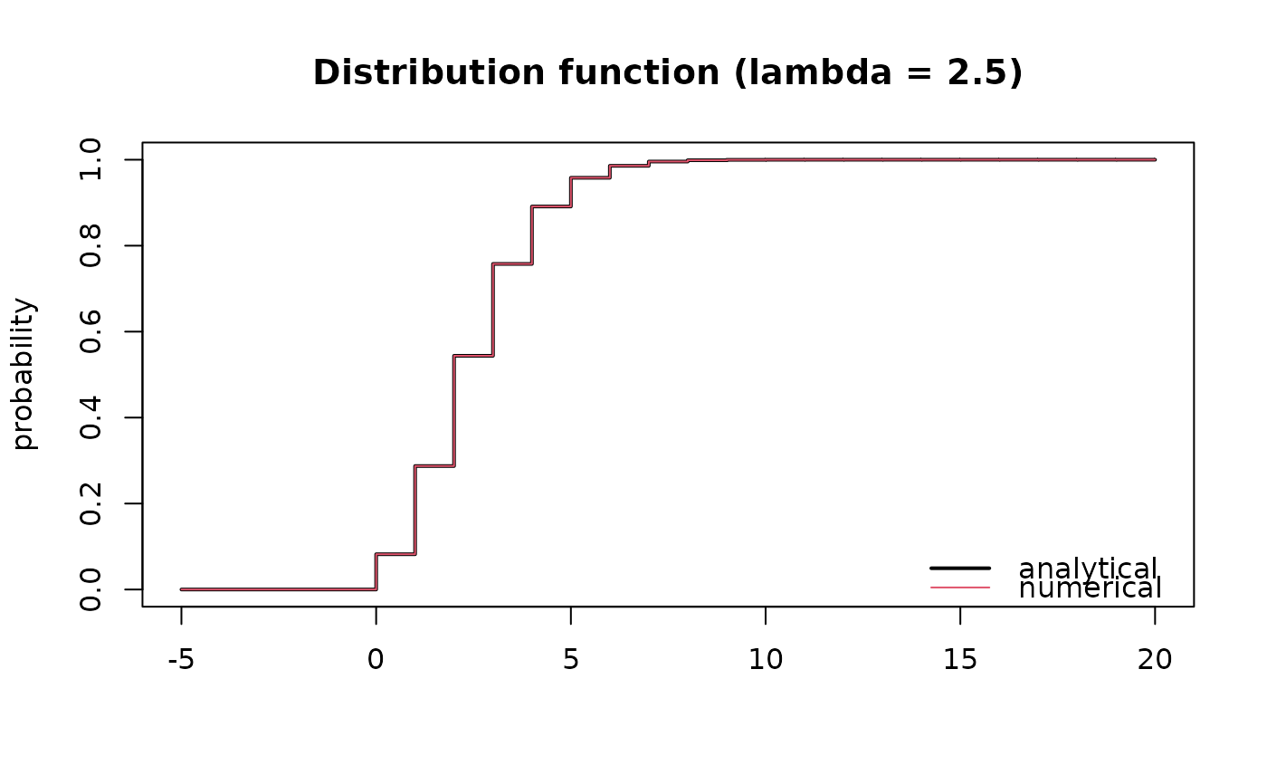
## Visual comparison: distribution function
x <- seq(-5, 20, by = 1)
dcdf <- data.frame(x = x,
analytical = cdf(p3[2L], x = x),
numerical = cdf(mp3[2L], x = x))
matplot(dcdf[, 1], dcdf[, -1], type = "s", col = 1:2,
xlab = NA, ylab = "probability",
lty = 1, lwd = 2:1, main = "Distribution function (lambda = 2.5)")
legend("bottomright", legend = names(dcdf)[-1], lty = 1,
col = 1:2, lwd = 2:1, bty = "n")
## ------------ custom Normal distribution (MyNormal2) ----------------
## ------------------- using pdf and quantile -------------------------
## Constructor function for new 'MyNormal2' distribution
MyNormal2 <- function(mu, sigma) {
d <- data.frame(mu = mu, sigma = sigma)
class(d) <- c("MyNormal2", "distribution")
return(d)
}
## Additionally required S3 methods (borrowed from class Normal)
registerS3method("pdf", "MyNormal2",
getS3method("pdf", class = "Normal"))
registerS3method("quantile", "MyNormal2",
getS3method("quantile", class = "Normal"))
registerS3method("is_discrete", "MyNormal2",
getS3method("is_discrete", class = "Normal"))
registerS3method("support", "MyNormal2",
getS3method("support", class = "Normal"))
## Constructing objects; creating three (named) 'MyNormal2' distributions
## with mean c(1, 2, 3) and standard deviation c(1, 2.5, 5) for which only
## pdf, quantile, is_discrete, and support are defined.
mn3 <- MyNormal2(mu = 1:3, sigma = c(1, 2.5, 5))
mn3 <- setNames(mn3, LETTERS[1:3])
random(mn3, n = 3L)
#> r_1 r_2 r_3
#> A -0.1116676 1.3159445 1.946852
#> B 1.4714667 -0.8035612 -2.571860
#> C -7.7730979 3.3825496 -1.126420
cdf(mn3, x = 2)
#> A B C
#> 0.8413448 0.5000000 0.4207403
pdf(mn3, x = 2)
#> A B C
#> 0.24197072 0.15957691 0.07820854
quantile(mn3, 0.5)
#> A B C
#> 1 2 3
cbind(mean = mean(mn3), variance = variance(mn3),
skewness = skewness(mn3), kurtosis = kurtosis(mn3))
#> mean variance skewness kurtosis
#> A 1 1.002989 2.667538e-15 0.0349172
#> B 2 6.268683 4.534914e-15 0.0349172
#> C 3 25.074732 4.563209e-15 0.0349172
# \donttest{
## ------------ custom Poisson distribution (MyPoisson1) --------------
## -------------------------- using pdf -------------------------------
## Custom constructor function for the 'MyPoisson1' distribution
MyPoisson1 <- function(lambda) {
d <- data.frame(lambda = lambda)
class(d) <- c("MyPoisson1", "distribution")
return(d)
}
## Additionally required S3 methods (borrowed from class Poisson)
registerS3method("pdf", "MyPoisson1",
getS3method("pdf", class = "Poisson"))
registerS3method("is_discrete", "MyPoisson1",
getS3method("is_discrete", class = "Poisson"))
registerS3method("support", "MyPoisson1",
getS3method("support", class = "Poisson"))
## Constructing objects; three normal distributions with
## parameter lambda = c(1, 2.5, 5).
## mp3: Based on MyPoisson1 where only pdf, id_discrete, and support
## are defined.
## p3: Analytic solution (Poisson()) with analytic
## functions for all distribution functions (pdf, cdf, quantile)
## as well as for the first four central moments (mean,
## variance, skewness, kurtosis)
mp3 <- MyPoisson1(lambda = c(1, 2.5, 5))
p3 <- Poisson(lambda = c(1, 2.5, 5))
## Class 'MyPoisson1' knows the analytic cdf:
pdf(mp3, x = 2)
#> [1] 0.18393972 0.25651562 0.08422434
identical(pdf(mp3, x = 2), pdf(p3, x = 2))
#> [1] TRUE
## Calculating distribution at x = 2
cdf(mp3, x = 2) ## Numeric approximation
#> [1] 0.9196986 0.5438131 0.1246520
cdf(mp3, x = 2) ## Analytic solution
#> [1] 0.9196986 0.5438131 0.1246520
cdf(mp3, x = 2) - cdf(p3, x = 2) ## Pairwise differences/precision
#> [1] 0.000000e+00 0.000000e+00 -1.387779e-17
## Calculating quantiles
probs <- c(0.0, 0.01, 0.25, 0.5, 0.75, 0.99, 1.0)
quantile(mp3, probs = probs) ## Numeric approximation
#> q_0 q_0.01 q_0.25 q_0.5 q_0.75 q_0.99 q_1
#> [1,] 0 0 0 1 2 4 Inf
#> [2,] 0 0 1 2 3 7 Inf
#> [3,] 0 1 3 5 6 11 Inf
quantile(p3, probs = probs) ## Analytic solution
#> q_0 q_0.01 q_0.25 q_0.5 q_0.75 q_0.99 q_1
#> [1,] 0 0 0 1 2 4 Inf
#> [2,] 0 0 1 2 3 7 Inf
#> [3,] 0 1 3 5 6 11 Inf
probs2 <- seq(0.01, 0.99, by = 0.01)
qmp3 <- quantile(mp3, probs = probs2) ## Numeric approximation
qp3 <- quantile(p3, probs = probs2) ## Analytic solution
range(qmp3 - qp3) ## Range of pairwise differences/precision
#> [1] 0 0
## Central moments
cbind(mean = mean(mp3), variance = variance(mp3),
skewness = skewness(mp3), kurtosis = kurtosis(mp3))
#> mean variance skewness kurtosis
#> [1,] 1.0 1.000000 1.0000000 1.000000
#> [2,] 2.5 2.500000 0.6324555 0.400000
#> [3,] 5.0 4.999995 0.4472064 0.199942
## Visual comparison: distribution function
x <- seq(-5, 20, by = 1)
dcdf <- data.frame(x = x,
analytical = cdf(p3[2L], x = x),
numerical = cdf(mp3[2L], x = x))
matplot(dcdf[, 1], dcdf[, -1], type = "s", col = 1:2,
xlab = NA, ylab = "probability",
lty = 1, lwd = 2:1, main = "Distribution function (lambda = 2.5)")
legend("bottomright", legend = names(dcdf)[-1], lty = 1,
col = 1:2, lwd = 2:1, bty = "n")
 ## Visual comparison: quantile function
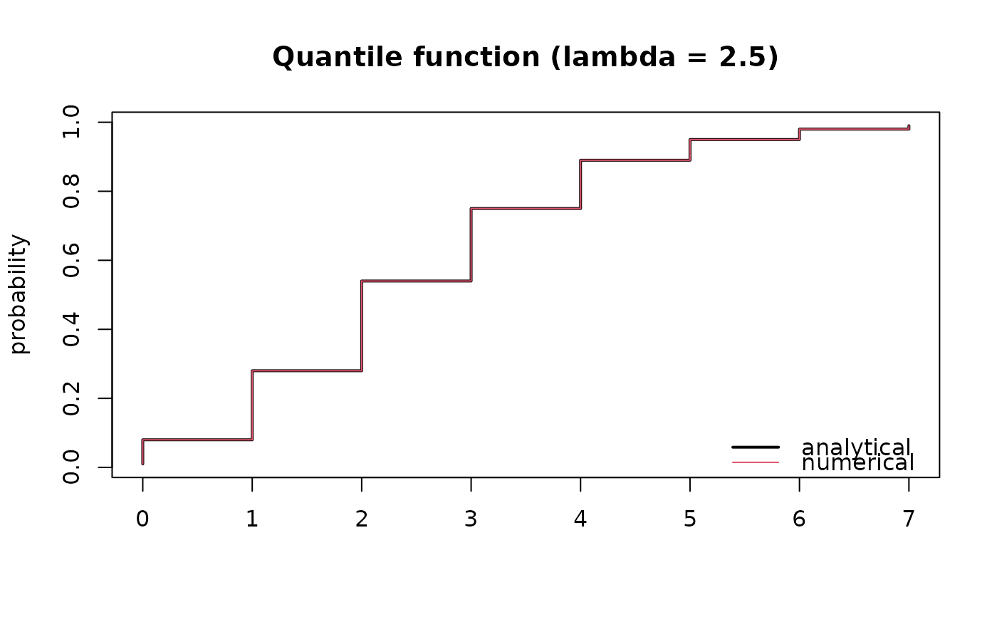
probs <- seq(0.01, 0.99, by = 0.01)
dquantile <- data.frame(probs = probs,
analytical = quantile(p3[2L], probs = probs),
numerical = quantile(mp3[2L], probs = probs))
matplot(dquantile[, -1], dquantile[, 1], type = "s", col = 1:2,
xlab = NA, ylab = "probability",
lty = 1, lwd = 2:1, main = "Quantile function (lambda = 2.5)")
legend("bottomright", legend = names(dquantile)[-1], lty = 1,
col = 1:2, lwd = 2:1, bty = "n")
## Visual comparison: quantile function
probs <- seq(0.01, 0.99, by = 0.01)
dquantile <- data.frame(probs = probs,
analytical = quantile(p3[2L], probs = probs),
numerical = quantile(mp3[2L], probs = probs))
matplot(dquantile[, -1], dquantile[, 1], type = "s", col = 1:2,
xlab = NA, ylab = "probability",
lty = 1, lwd = 2:1, main = "Quantile function (lambda = 2.5)")
legend("bottomright", legend = names(dquantile)[-1], lty = 1,
col = 1:2, lwd = 2:1, bty = "n")
 ## Quantile-Quantile plot
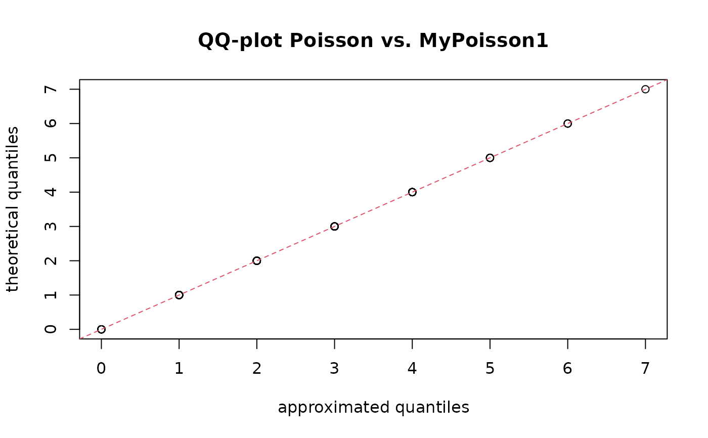
probs <- seq(0.01, 0.99, by = 0.01)
plot(quantile(p3[2], probs), quantile(mp3[2], probs),
main = "QQ-plot Poisson vs. MyPoisson1",
xlab = "approximated quantiles", ylab = "theoretical quantiles")
abline(0, 1, col = 2, lty = 2)
## Quantile-Quantile plot
probs <- seq(0.01, 0.99, by = 0.01)
plot(quantile(p3[2], probs), quantile(mp3[2], probs),
main = "QQ-plot Poisson vs. MyPoisson1",
xlab = "approximated quantiles", ylab = "theoretical quantiles")
abline(0, 1, col = 2, lty = 2)
 ## Drawing random numbers (200 on third distribution)
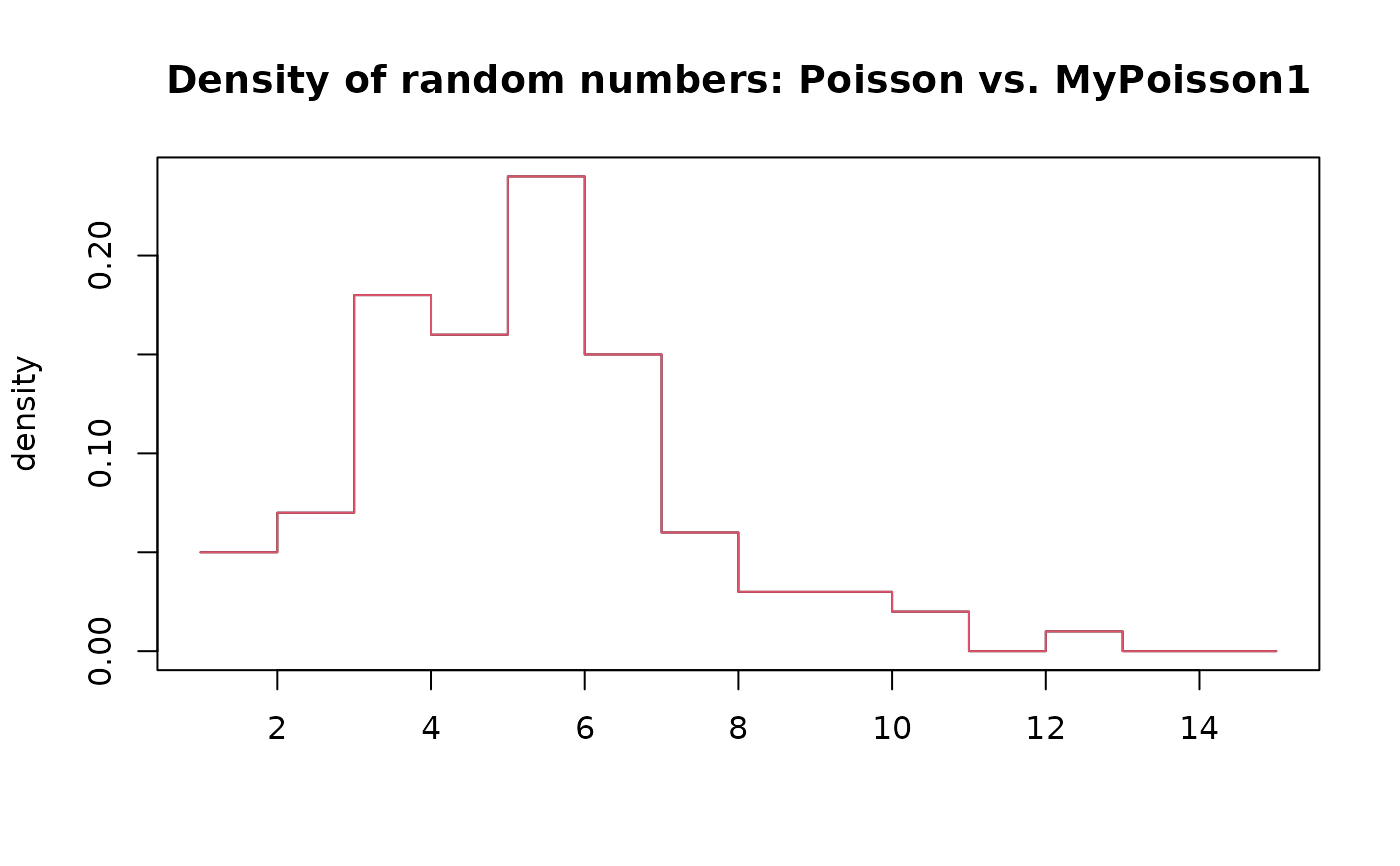
set.seed(6020); rmp <- random(mp3[3], 100L)
set.seed(6020); rp <- random(p3[3], 100L)
hmp <- hist(rmp, breaks = 0:15, plot = FALSE)
hp <- hist(rp, breaks = 0:15, plot = FALSE)
plot(hmp$breaks[-1], hmp$density, type = "s",
xlab = NA, ylab = "density",
main = "Density of random numbers: Poisson vs. MyPoisson1")
lines(hp$breaks[-1], hp$density, col = 2, type = "s")
## Drawing random numbers (200 on third distribution)
set.seed(6020); rmp <- random(mp3[3], 100L)
set.seed(6020); rp <- random(p3[3], 100L)
hmp <- hist(rmp, breaks = 0:15, plot = FALSE)
hp <- hist(rp, breaks = 0:15, plot = FALSE)
plot(hmp$breaks[-1], hmp$density, type = "s",
xlab = NA, ylab = "density",
main = "Density of random numbers: Poisson vs. MyPoisson1")
lines(hp$breaks[-1], hp$density, col = 2, type = "s")
 ## ------------ custom Poisson distribution (MyPoisson2) --------------
## -------------------------- using cdf -------------------------------
## Custom constructor function for the 'MyPoisson2' distribution
MyPoisson2 <- function(lambda) {
d <- data.frame(lambda = lambda)
class(d) <- c("MyPoisson2", "distribution")
return(d)
}
## Additionally required S3 methods (borrowed from class Poisson)
registerS3method("cdf", "MyPoisson2",
getS3method("cdf", class = "Poisson"))
registerS3method("is_discrete", "MyPoisson2",
getS3method("is_discrete", class = "Poisson"))
registerS3method("support", "MyPoisson2",
getS3method("support", class = "Poisson"))
## Constructing objects; creating three (named) 'MyPoisson2' distributions
## with lambda c(1, 2.5, 5) for which only cdf, is_discrete,
## and support are defined.
mp3 <- MyPoisson2(lambda = c(1, 2.5, 5))
mp3 <- setNames(mp3, LETTERS[4:6])
random(mp3, n = 3L)
#> r_1 r_2 r_3
#> D 1 1 0
#> E 0 2 3
#> F 6 4 7
cdf(p3, x = 2)
#> [1] 0.9196986 0.5438131 0.1246520
pdf(p3, x = 2)
#> [1] 0.18393972 0.25651562 0.08422434
quantile(p3, 0.5)
#> [1] 1 2 5
cbind(mean = mean(p3), variance = variance(p3),
skewness = skewness(p3), kurtosis = kurtosis(p3))
#> mean variance skewness kurtosis
#> [1,] 1.0 1.0 1.0000000 1.0
#> [2,] 2.5 2.5 0.6324555 0.4
#> [3,] 5.0 5.0 0.4472136 0.2
# }
## ------------ custom Poisson distribution (MyPoisson2) --------------
## -------------------------- using cdf -------------------------------
## Custom constructor function for the 'MyPoisson2' distribution
MyPoisson2 <- function(lambda) {
d <- data.frame(lambda = lambda)
class(d) <- c("MyPoisson2", "distribution")
return(d)
}
## Additionally required S3 methods (borrowed from class Poisson)
registerS3method("cdf", "MyPoisson2",
getS3method("cdf", class = "Poisson"))
registerS3method("is_discrete", "MyPoisson2",
getS3method("is_discrete", class = "Poisson"))
registerS3method("support", "MyPoisson2",
getS3method("support", class = "Poisson"))
## Constructing objects; creating three (named) 'MyPoisson2' distributions
## with lambda c(1, 2.5, 5) for which only cdf, is_discrete,
## and support are defined.
mp3 <- MyPoisson2(lambda = c(1, 2.5, 5))
mp3 <- setNames(mp3, LETTERS[4:6])
random(mp3, n = 3L)
#> r_1 r_2 r_3
#> D 1 1 0
#> E 0 2 3
#> F 6 4 7
cdf(p3, x = 2)
#> [1] 0.9196986 0.5438131 0.1246520
pdf(p3, x = 2)
#> [1] 0.18393972 0.25651562 0.08422434
quantile(p3, 0.5)
#> [1] 1 2 5
cbind(mean = mean(p3), variance = variance(p3),
skewness = skewness(p3), kurtosis = kurtosis(p3))
#> mean variance skewness kurtosis
#> [1,] 1.0 1.0 1.0000000 1.0
#> [2,] 2.5 2.5 0.6324555 0.4
#> [3,] 5.0 5.0 0.4472136 0.2
# }