Generic functions and methods for computing score and Hessian
Source:R/Bernoulli.R, R/Binomial.R, R/Normal.R, and 4 more
score-hessian.RdThe generic functions score and hessian along with the corresponding
methods for distribution objects enable the computation of the
score (first derivative of the log-likelihood with respect to the
parameters) and Hessian (corresponding second derivative).
Usage
score(d, ...)

hessian(d, ...)

# S3 method for class 'distribution'
score(d, x, which = NULL, drop = TRUE, eps = .Machine$double.eps^(1/3), ...)

# S3 method for class 'distribution'
hessian(
  d,
  x,
  which = NULL,
  drop = TRUE,
  expected = FALSE,
  eps = .Machine$double.eps^(1/4),
  ...
)
Arguments
- d
An object, typically a distribution object, e.g., as created by
Normal()orBinomial().- x
A vector of elements whose score/Hessian should be determined given the distribution
d. Eitherdandxneed to have the same length or length 1.- which
character or
NULL(default). Character labels for the derivatives to be included in the score or Hessian respectively. Inscorethe possible values are (combinations of) the parameter names (e.g.,"mu"and/or"sigma"). Inhessianadditionally the cross-derivatives (e.g.,mu:sigmaandsigma:mu) are available. By default (ifwhich = NULL) all elements of the score or Hessian should be computed.- drop
logical. Should the result be simplified to a vector if possible?
- ...
Arguments passed to methods.
- expected
logical. Should the expected Hessian be computed? If
FALSEthe observed Hessian is computed. Some methods might only support only one or the the other option and defaults might differ.- eps
numeric. Tolerance when obtaining the score or Hessian via numeric differentiation.
Value
Either a numeric matrix with suitable column names is returned or a numeric
vector (provided that which has length 1 and drop = TRUE).
Details
In the methods for dedicated distributions analytical results for computing
the score or Hessian should be used. All hessian methods should implemented
the expected argument with an appropriate default. If a hessian method only
supports the expected or the observed Hessian, then an error should be issued
if needed.
In the fallback methods for general distribution objects a simple differencing
approach is used. Either differences of log_pdf (for the score) or of
score (for the hessian) with slightly modified parameters are used. If
the parameters in a distribution are on the boundary of the parameter space
this might lead to errors in the computation.
Examples
X <- Normal(mu = c(0, 1, 2), sigma = c(2, 1, 1))
x <- c(0, 0, 1)
score(X, x)
#> mu sigma
#> [1,] 0 -0.5
#> [2,] -1 0.0
#> [3,] -1 0.0
hessian(X, x)
#> mu sigma:mu mu:sigma sigma
#> [1,] -0.25 0 0 0.25
#> [2,] -1.00 2 2 -2.00
#> [3,] -1.00 2 2 -2.00
hessian(X, x, expected = TRUE)
#> mu sigma:mu mu:sigma sigma
#> [1,] -0.25 0 0 -0.5
#> [2,] -1.00 0 0 -2.0
#> [3,] -1.00 0 0 -2.0
h <- hessian(X[1], x[1], expected = TRUE)
matrix(h, ncol = 2, dimnames = list(c("mu", "sigma"), c("mu", "sigma")))
#> mu sigma
#> mu -0.25 0.0
#> sigma 0.00 -0.5
## Comparison of analytic and numeric score/Hessian (Normal(3, 2))
X <- Normal(mu = 3, sigma = 2)
x <- seq(0, 6, by = 0.01)
#' ## score: derivative of log-likelihood by parameter sigma
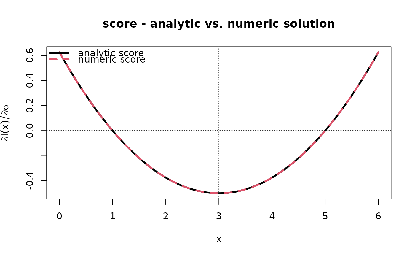
s_analytic <- score(X, x, which = "sigma")
s_numeric <- distributions3:::score.distribution(X, x, which = "sigma")
message("Sum of absolute differences (score): ", sum(abs(s_analytic - s_numeric)))
#> Sum of absolute differences (score): 9.21342668477876e-09
matplot(x, cbind(s_analytic, s_numeric), col = 1:2, type = "l", lty = 1:2,
lwd = 3, xlab = "x", main = "score - analytic vs. numeric solution",
ylab = expression(partialdiff * l(x) / partialdiff * sigma))
legend("topleft", legend = c("analytic score", "numeric score"),
bty = "n", pch = NA, lty = 1:2, col = 1:2, lwd = 3)
abline(h = 0, v = 3, lty = 3)
 #' ## Hessian: second derivative of log-likelihood by sigma^2
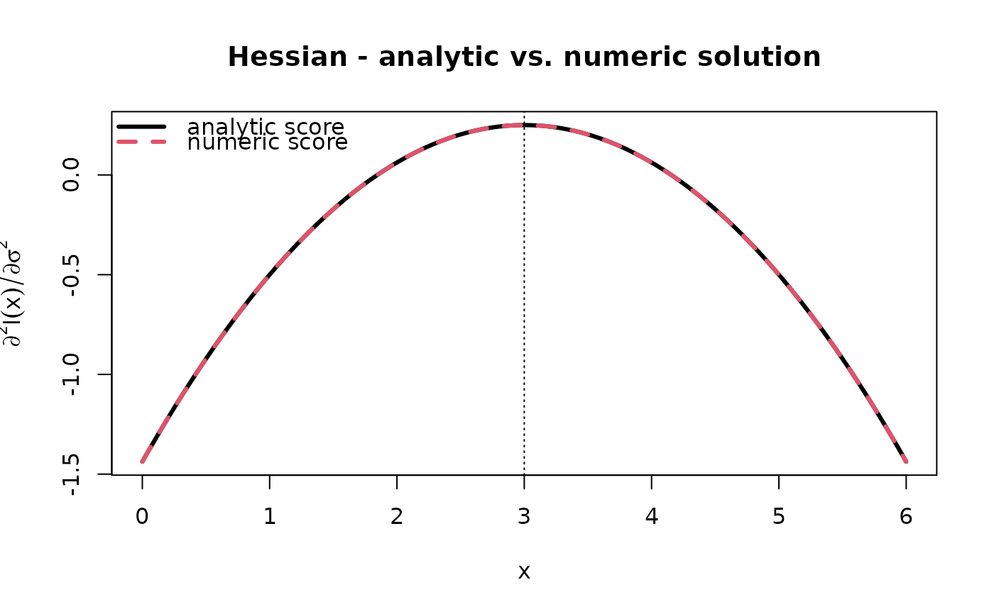
h_analytic <- hessian(X, x, which = "sigma")
h_numeric <- distributions3:::hessian.distribution(X, x, which = "sigma")
message("Sum of absolute differences (Hessian): ", sum(abs(h_analytic - h_numeric)))
#> Sum of absolute differences (Hessian): 3.80928397653024e-06
matplot(x, cbind(h_analytic, h_numeric), col = 1:2, type = "l", lty = 1:2,
lwd = 3, xlab = "x", main = "Hessian - analytic vs. numeric solution",
ylab = expression(partialdiff^2 * l(x) / partialdiff * sigma^2))
legend("topleft", legend = c("analytic score", "numeric score"),
bty = "n", pch = NA, lty = 1:2, col = 1:2, lwd = 3)
abline(v = 3, lty = 3)
#' ## Hessian: second derivative of log-likelihood by sigma^2
h_analytic <- hessian(X, x, which = "sigma")
h_numeric <- distributions3:::hessian.distribution(X, x, which = "sigma")
message("Sum of absolute differences (Hessian): ", sum(abs(h_analytic - h_numeric)))
#> Sum of absolute differences (Hessian): 3.80928397653024e-06
matplot(x, cbind(h_analytic, h_numeric), col = 1:2, type = "l", lty = 1:2,
lwd = 3, xlab = "x", main = "Hessian - analytic vs. numeric solution",
ylab = expression(partialdiff^2 * l(x) / partialdiff * sigma^2))
legend("topleft", legend = c("analytic score", "numeric score"),
bty = "n", pch = NA, lty = 1:2, col = 1:2, lwd = 3)
abline(v = 3, lty = 3)