Deletion and Other Diagnostic Methods for "ivreg" Objects
Source: R/ivregDiagnostics.R
ivregDiagnostics.RdMethods for computing deletion and other regression diagnostics for 2SLS regression.
It's generally more efficient to compute the deletion diagnostics via the influence
method and then to extract the various specific diagnostics with the methods for
"influence.ivreg" objects. Other diagnostics for linear models, such as
added-variable plots (avPlots) and component-plus-residual
plots (crPlots), also work, as do effect plots
(e.g., predictorEffects) with residuals (see the examples below).
The pointwise confidence envelope for the qqPlot method assumes an independent random sample
from the t distribution with degrees of freedom equal to the residual degrees of
freedom for the model and so are approximate, because the studentized residuals aren't
independent.
For additional information, see the vignette Diagnostics for 2SLS Regression.
# S3 method for class 'ivreg'
influence(
  model,
  sigma. = n <= 1000,
  type = c("stage2", "both", "maximum"),
  applyfun = NULL,
  ncores = NULL,
  ...
)

# S3 method for class 'ivreg'
rstudent(model, ...)

# S3 method for class 'ivreg'
cooks.distance(model, ...)

# S3 method for class 'influence.ivreg'
dfbeta(model, ...)

# S3 method for class 'ivreg'
dfbeta(model, ...)

# S3 method for class 'ivreg'
hatvalues(model, type = c("stage2", "both", "maximum", "stage1"), ...)

# S3 method for class 'influence.ivreg'
rstudent(model, ...)

# S3 method for class 'influence.ivreg'
hatvalues(model, ...)

# S3 method for class 'influence.ivreg'
cooks.distance(model, ...)

# S3 method for class 'influence.ivreg'
qqPlot(
  x,
  ylab = paste("Studentized Residuals(", deparse(substitute(x)), ")", sep = ""),
  distribution = c("t", "norm"),
  ...
)

# S3 method for class 'ivreg'
influencePlot(model, ...)

# S3 method for class 'influence.ivreg'
influencePlot(model, ...)

# S3 method for class 'ivreg'
infIndexPlot(model, ...)

# S3 method for class 'influence.ivreg'
infIndexPlot(model, ...)

# S3 method for class 'influence.ivreg'
model.matrix(object, ...)

# S3 method for class 'ivreg'
avPlots(model, terms, ...)

# S3 method for class 'ivreg'
avPlot(model, ...)

# S3 method for class 'ivreg'
mcPlots(model, terms, ...)

# S3 method for class 'ivreg'
mcPlot(model, ...)

# S3 method for class 'ivreg'
Boot(
  object,
  f = coef,
  labels = names(f(object)),
  R = 999,
  method = "case",
  ncores = 1,
  ...
)

# S3 method for class 'ivreg'
crPlots(model, terms, ...)

# S3 method for class 'ivreg'
crPlot(model, ...)

# S3 method for class 'ivreg'
ceresPlots(model, terms, ...)

# S3 method for class 'ivreg'
ceresPlot(model, ...)

# S3 method for class 'ivreg'
plot(x, ...)

# S3 method for class 'ivreg'
qqPlot(x, distribution = c("t", "norm"), ...)

# S3 method for class 'ivreg'
outlierTest(model, ...)

# S3 method for class 'ivreg'
spreadLevelPlot(x, main = "Spread-Level Plot", ...)

# S3 method for class 'ivreg'
ncvTest(model, ...)

# S3 method for class 'ivreg'
deviance(object, ...)

# S3 method for class 'rivreg'
influence(model, ...)
Arguments
- model, x, object
A
"ivreg"or"influence.ivreg"object.- sigma.
If
TRUE(the default for 1000 or fewer cases), the deleted value of the residual standard deviation is computed for each case; ifFALSE, the overall residual standard deviation is used to compute other deletion diagnostics.- type
If
"stage2"(the default), hatvalues are for the second stage regression; if"both", the hatvalues are the geometric mean of the casewise hatvalues for the two stages; if"maximum", the hatvalues are the larger of the casewise hatvalues for the two stages. In computing the geometric mean or casewise maximum hatvalues, the hatvalues for each stage are first divided by their average (number of coefficients in stage regression/number of cases); the geometric mean or casewise maximum values are then multiplied by the average hatvalue from the second stage.- applyfun
Optional loop replacement function that should work like
lapplywith argumentsfunction(X, FUN, ...). The default is to use a loop unless thencoresargument is specified (see below).- ncores
Numeric, number of cores to be used in parallel computations. If set to an integer the
applyfunis set to use eitherparLapply(on Windows) ormclapply(otherwise) with the desired number of cores.- ...
arguments to be passed down.
- ylab
The vertical axis label.
- distribution
"t"(the default) or"norm".- terms
Terms for which added-variable plots are to be constructed; the default, if the argument isn't specified, is the
"regressors"component of the model formula.- f, labels, R
see
Boot.- method
only
"case"(case resampling) is supported: seeBoot.- main
Main title for the graph.
Value
In the case of influence.ivreg, an object of class "influence.ivreg"
with the following components:
coefficientsthe estimated regression coefficients
modelthe model matrix
dfbetainfluence on coefficients
sigmadeleted values of the residual standard deviation
dffitsoverall influence on the regression coefficients
cookdCook's distances
hatvalueshatvalues
rstudentStudentized residuals
df.residualresidual degrees of freedom
In the case of other methods, such as rstudent.ivreg or
rstudent.influence.ivreg, the corresponding diagnostic statistics.
Many other methods (e.g., crPlot.ivreg, avPlot.ivreg, Effect.ivreg)
draw graphs.
See also
Examples
kmenta.eq1 <- ivreg(Q ~ P + D | D + F + A, data = Kmenta)
summary(kmenta.eq1)
#>
#> Call:
#> ivreg(formula = Q ~ P + D | D + F + A, data = Kmenta)
#>
#> Residuals:
#> Min 1Q Median 3Q Max
#> -3.4305 -1.2432 -0.1895 1.5762 2.4920
#>
#> Coefficients:
#> Estimate Std. Error t value Pr(>|t|)
#> (Intercept) 94.63330 7.92084 11.947 1.08e-09 ***
#> P -0.24356 0.09648 -2.524 0.0218 *
#> D 0.31399 0.04694 6.689 3.81e-06 ***
#> ---
#> Signif. codes: 0 ‘***’ 0.001 ‘**’ 0.01 ‘*’ 0.05 ‘.’ 0.1 ‘ ’ 1
#>
#> Residual standard error: 1.966 on 17 degrees of freedom
#> Multiple R-Squared: 0.7548, Adjusted R-squared: 0.726
#> Wald test: 23.81 on 2 and 17 DF, p-value: 1.178e-05
#>
car::avPlots(kmenta.eq1)
#> Error in avPlot.lm(model, term, main = "", ...): P is not a column of the model matrix.
car::mcPlots(kmenta.eq1)
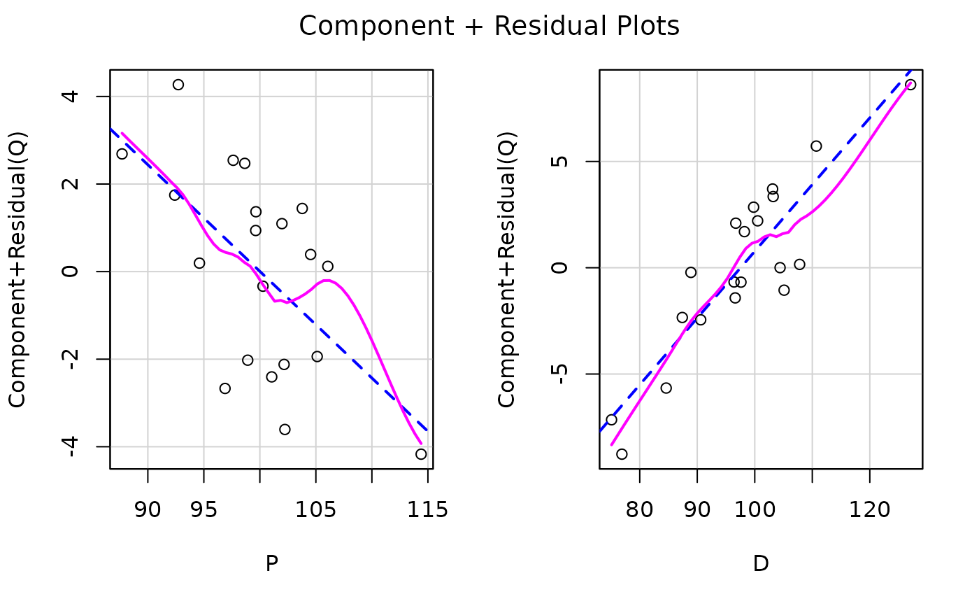
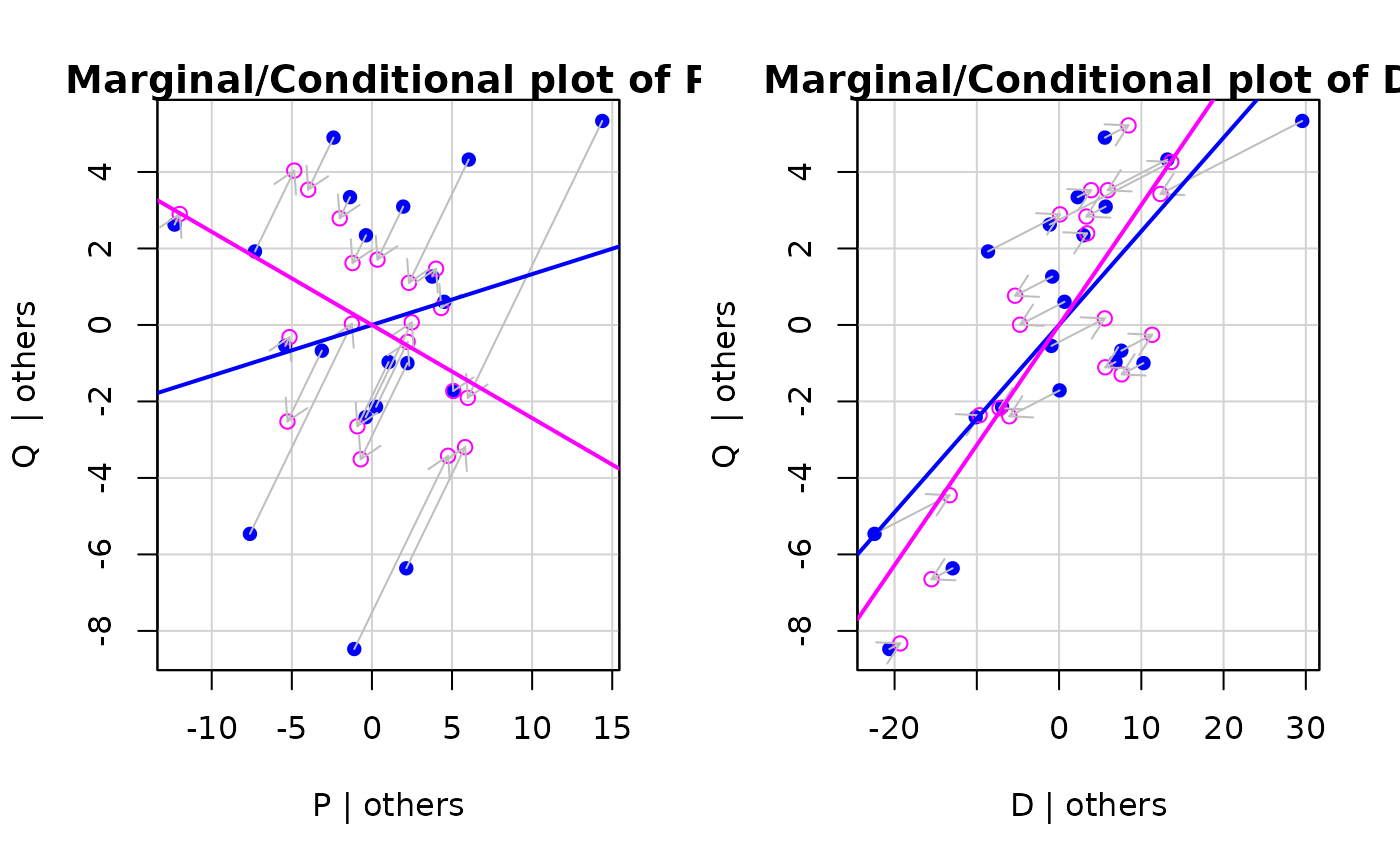 car::crPlots(kmenta.eq1)
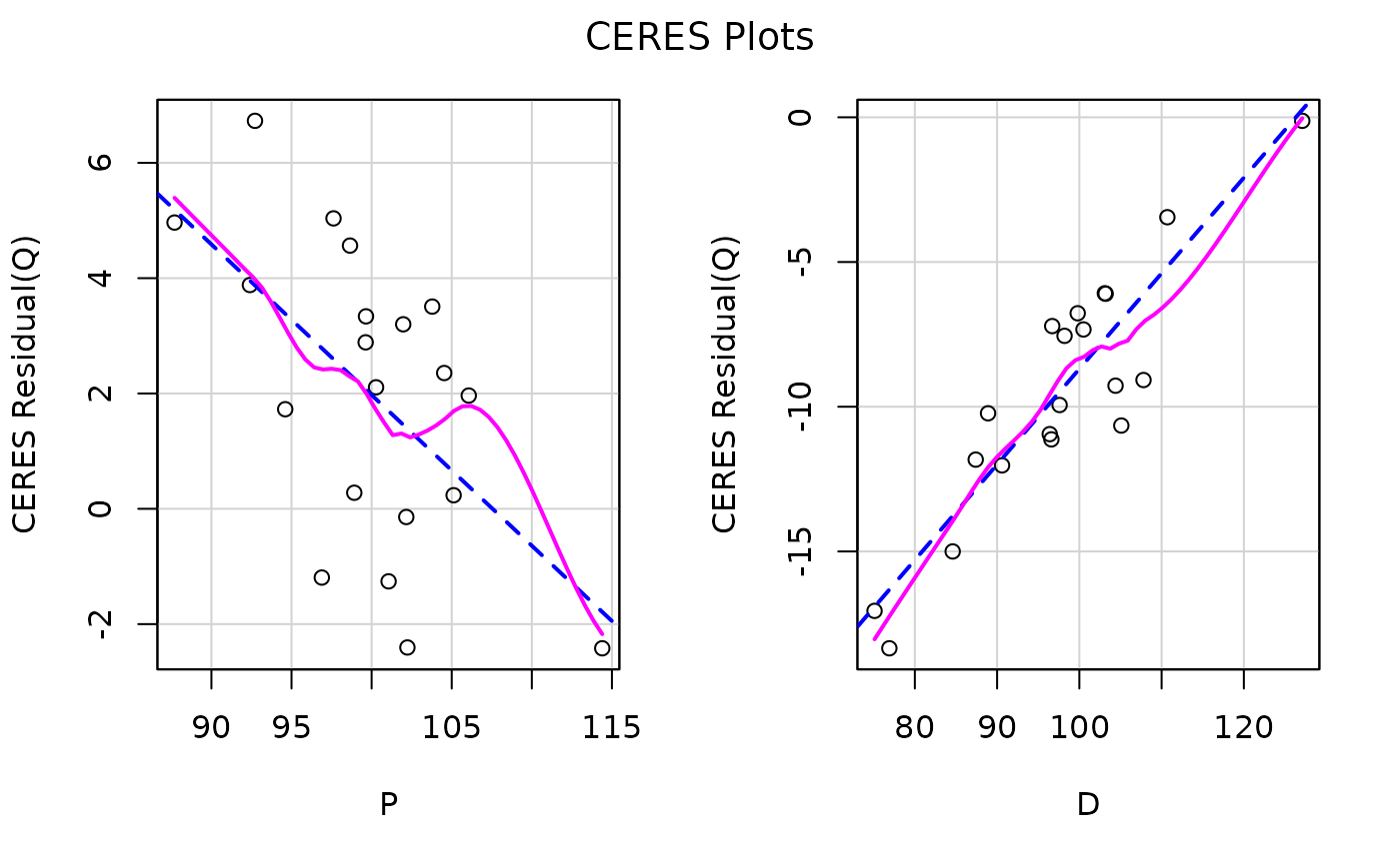
 car::ceresPlots(kmenta.eq1)
 car::influencePlot(kmenta.eq1)
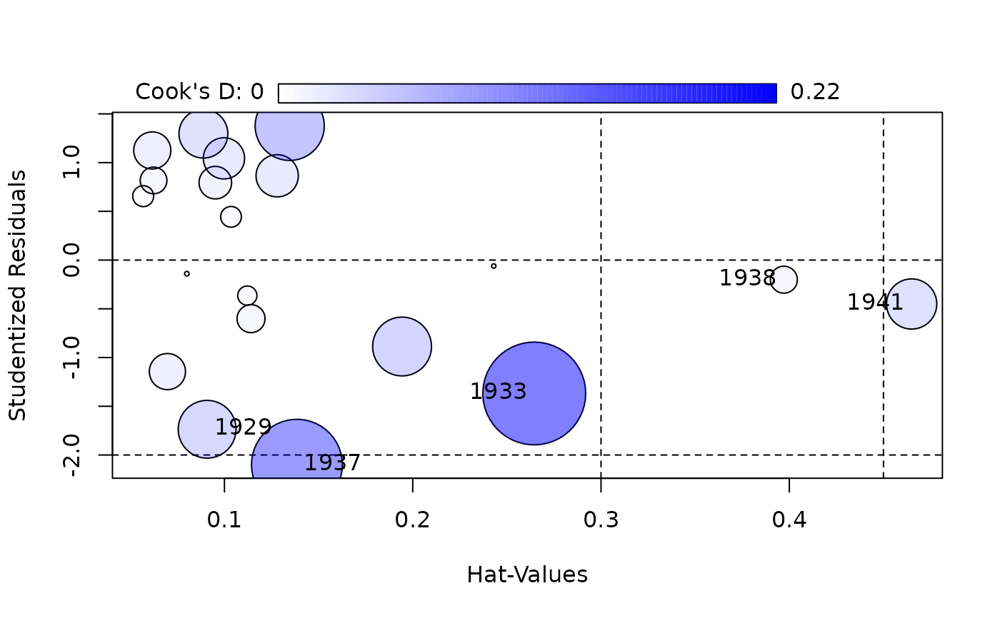 #> StudRes Hat CookD
#> 1 -1.7359357 0.09079703 0.06956671
#> 2 -1.3686682 0.26453459 0.21973049
#> 3 -2.0995532 0.13849570 0.17147564
#> 4 -0.2010944 0.39711512 0.01508349
#> 5 -0.4505155 0.46498004 0.05257374
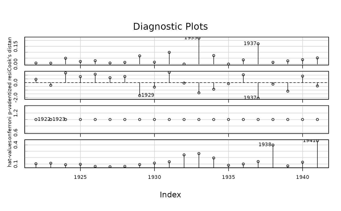
car::influenceIndexPlot(kmenta.eq1)
#> StudRes Hat CookD
#> 1 -1.7359357 0.09079703 0.06956671
#> 2 -1.3686682 0.26453459 0.21973049
#> 3 -2.0995532 0.13849570 0.17147564
#> 4 -0.2010944 0.39711512 0.01508349
#> 5 -0.4505155 0.46498004 0.05257374
car::influenceIndexPlot(kmenta.eq1)
 car::qqPlot(kmenta.eq1)
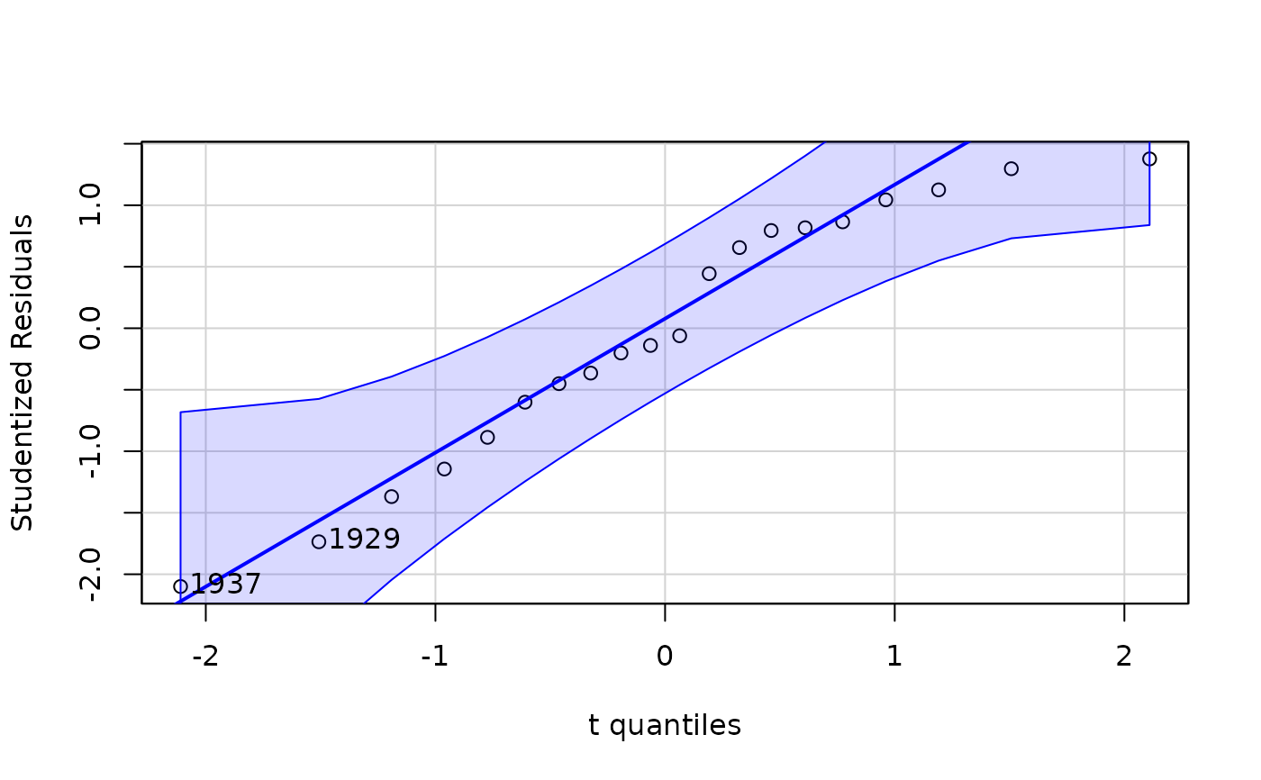 #> 1937 1929
#> 16 8
car::spreadLevelPlot(kmenta.eq1)
#> 1937 1929
#> 16 8
car::spreadLevelPlot(kmenta.eq1)
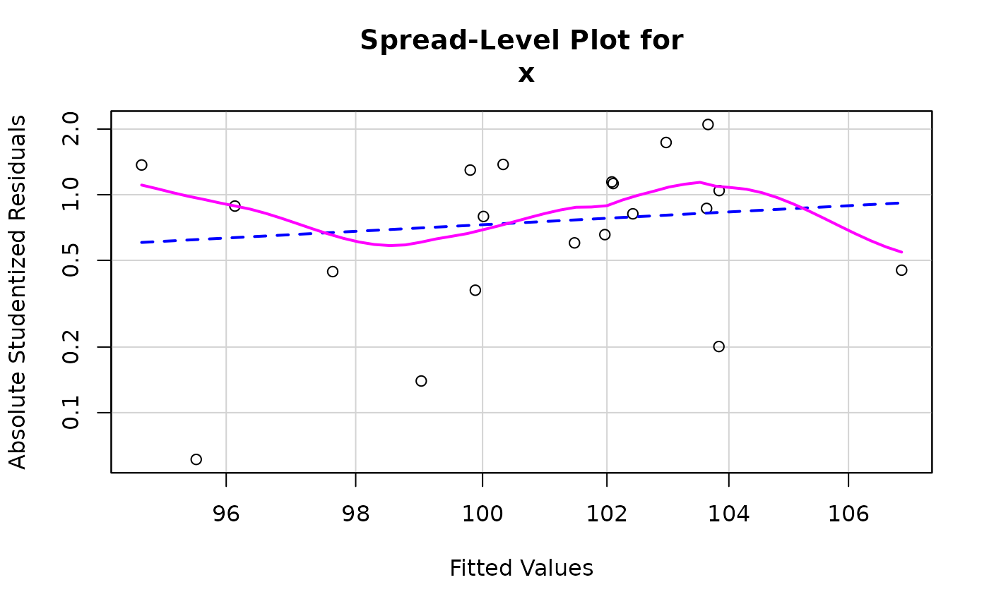 #>
#> Suggested power transformation: -2.44685
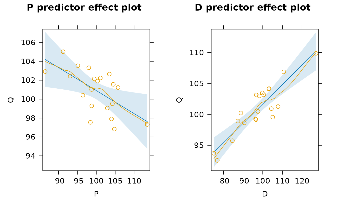
plot(effects::predictorEffects(kmenta.eq1, residuals = TRUE))
#>
#> Suggested power transformation: -2.44685
plot(effects::predictorEffects(kmenta.eq1, residuals = TRUE))
 set.seed <- 12321 # for reproducibility
confint(car::Boot(kmenta.eq1, R = 250)) # 250 reps for brevity
#> Bootstrap bca confidence intervals
#>
#> 2.5 % 97.5 %
#> (Intercept) 74.1021451 107.77780398
#> P -0.4454188 0.02161098
#> D 0.1902243 0.40024278
car::outlierTest(kmenta.eq1)
#> No Studentized residuals with Bonferroni p < 0.05
#> Largest |rstudent|:
#> rstudent unadjusted p-value Bonferroni p
#> 1937 -2.099553 0.051985 NA
car::ncvTest(kmenta.eq1)
#> Non-constant Variance Score Test
#> Variance formula: ~ fitted.values
#> Chisquare = 0.2390325, Df = 1, p = 0.62491
set.seed <- 12321 # for reproducibility
confint(car::Boot(kmenta.eq1, R = 250)) # 250 reps for brevity
#> Bootstrap bca confidence intervals
#>
#> 2.5 % 97.5 %
#> (Intercept) 74.1021451 107.77780398
#> P -0.4454188 0.02161098
#> D 0.1902243 0.40024278
car::outlierTest(kmenta.eq1)
#> No Studentized residuals with Bonferroni p < 0.05
#> Largest |rstudent|:
#> rstudent unadjusted p-value Bonferroni p
#> 1937 -2.099553 0.051985 NA
car::ncvTest(kmenta.eq1)
#> Non-constant Variance Score Test
#> Variance formula: ~ fitted.values
#> Chisquare = 0.2390325, Df = 1, p = 0.62491