Please see the documentation of SinhArcsinh() for some properties
of the Sinh-Arcsinh distribution, as well as extensive examples
showing to how calculate p-values and confidence intervals.
quantile()
Usage
# S3 method for class 'SinhArcsinh'
quantile(x, probs, drop = TRUE, elementwise = NULL, cores = NULL, ...)
Arguments
- x
A
SinhArcsinhobject created by a call toSinhArcsinh().- probs
A vector of probabilities.
- drop
logical. Should the result be simplified to a vector if possible?
- elementwise
logical. Should each distribution in
xbe evaluated at all elements ofprobs(elementwise = FALSE, yielding a matrix)? Or, ifxandprobshave the same length, should the evaluation be done element by element (elementwise = TRUE, yielding a vector)? The default ofNULLmeans thatelementwise = TRUEis used if the lengths match and otherwiseelementwise = FALSEis used.- cores
NULLor positive integer. TODO(R): Just a development option. If notNULLwe use the C code withcoresthreads.- ...
Arguments to be passed to
qnorm. Unevaluated arguments will generate a warning to catch mispellings or other possible errors.
Value
In case of a single distribution object, either a numeric
vector of length probs (if drop = TRUE, default) or a matrix with
length(probs) columns (if drop = FALSE). In case of a vectorized
distribution object, a matrix with length(probs) columns containing all
possible combinations.
Details
This function returns the same values that you get from a Z-table. Note
quantile() is the inverse of cdf(). Please see the documentation of SinhArcsinh() for some properties
of the Sinh-Arcsinh distribution, as well as extensive examples
showing to how calculate p-values and confidence intervals.
See also
Other SinhArcsinh distribution:
cdf.SinhArcsinh(),
pdf.SinhArcsinh()
Examples
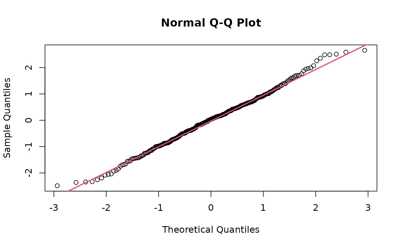
## SinhArcsinh() by default uses nu = 1, tau = 1 which
## results in the standard normal distribution
set.seed(6020)
X <- SinhArcsinh() # Uses mu = 1, sigma = 0, nu = 1, tau = 1)
x <- random(X, 300)
qqnorm(x); qqline(x, col = 2, lwd = 2)
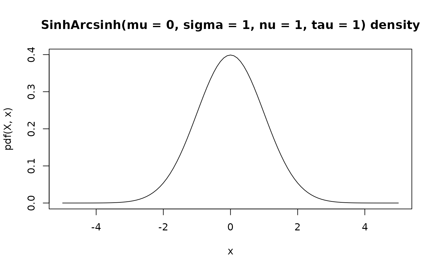
 curve(pdf(X, x), xlim = c(-5, 5), main = paste(X, "density"))
 ## Calculation of central moments is based on numeric integration,
## thus not being identical to the standard normal distribution
c(mean = mean(x), sd = sd(x))
#> mean sd
#> 0.001386471 0.999227517
## Skewed Sinh-Arcsinh distribution
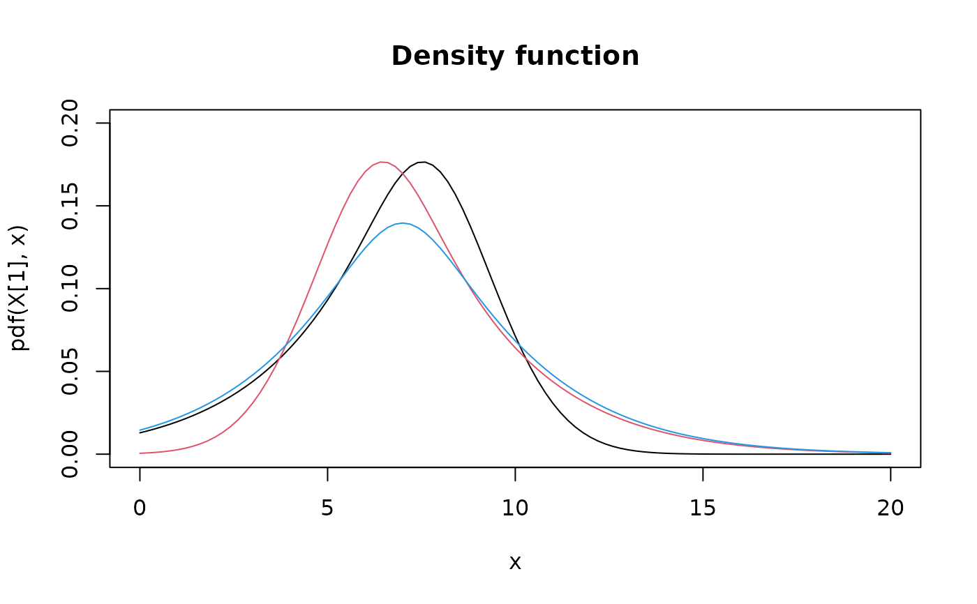
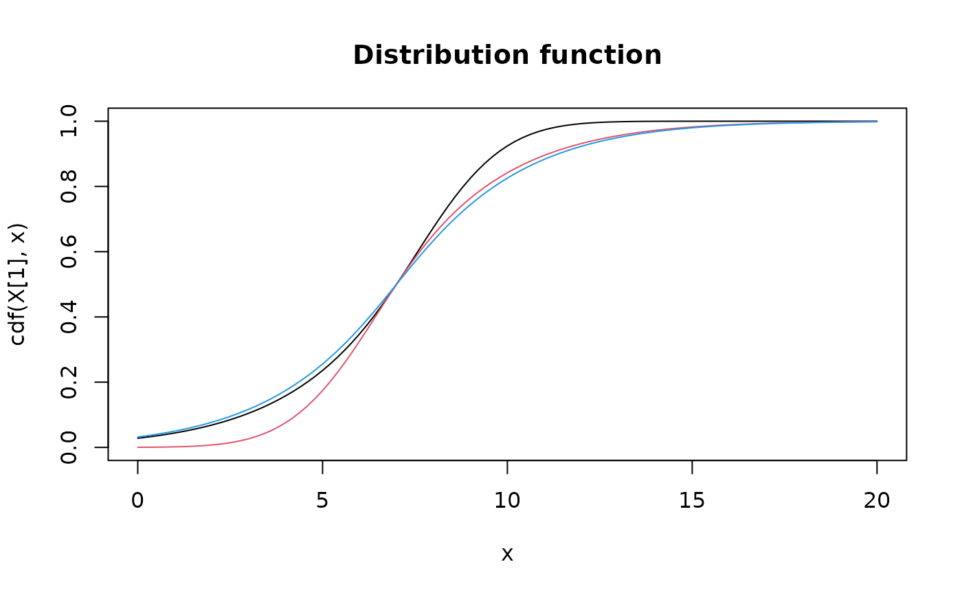
X <- SinhArcsinh(mu = 7, sigma = 2, nu = c(0.7, 1, 0.7), tau = c(1, 0.7, 0.7))
as.matrix(X)
#> mu sigma nu tau
#> [1,] 7 2 0.7 1.0
#> [2,] 7 2 1.0 0.7
#> [3,] 7 2 0.7 0.7
## Visualization of density functions using different parameters for nu/tau
curve(pdf(X[1], x), xlim = c(0, 20), ylim = c(0, 0.2), main = "Density function")
curve(pdf(X[2], x), xlim = c(0, 20), col = 2, add = TRUE)
curve(pdf(X[3], x), xlim = c(0, 20), col = 4, add = TRUE)
## Calculation of central moments is based on numeric integration,
## thus not being identical to the standard normal distribution
c(mean = mean(x), sd = sd(x))
#> mean sd
#> 0.001386471 0.999227517
## Skewed Sinh-Arcsinh distribution
X <- SinhArcsinh(mu = 7, sigma = 2, nu = c(0.7, 1, 0.7), tau = c(1, 0.7, 0.7))
as.matrix(X)
#> mu sigma nu tau
#> [1,] 7 2 0.7 1.0
#> [2,] 7 2 1.0 0.7
#> [3,] 7 2 0.7 0.7
## Visualization of density functions using different parameters for nu/tau
curve(pdf(X[1], x), xlim = c(0, 20), ylim = c(0, 0.2), main = "Density function")
curve(pdf(X[2], x), xlim = c(0, 20), col = 2, add = TRUE)
curve(pdf(X[3], x), xlim = c(0, 20), col = 4, add = TRUE)
 ## Visualization of distribution function using different parameters for nu/tau
curve(cdf(X[1], x), xlim = c(0, 20), ylim = 0:1, main = "Distribution function")
curve(cdf(X[2], x), xlim = c(0, 20), col = 2, add = TRUE)
curve(cdf(X[3], x), xlim = c(0, 20), col = 4, add = TRUE)
## Visualization of distribution function using different parameters for nu/tau
curve(cdf(X[1], x), xlim = c(0, 20), ylim = 0:1, main = "Distribution function")
curve(cdf(X[2], x), xlim = c(0, 20), col = 2, add = TRUE)
curve(cdf(X[3], x), xlim = c(0, 20), col = 4, add = TRUE)
 ## Central moments
mean(X)
#> [1] 6.579299 7.420701 7.000000
variance(X)
#> [1] 7.988051 7.988051 13.222747
skewness(X)
#> [1] -0.9964539 0.9964539 0.0000000
kurtosis(X)
#> [1] 1.986356 1.986356 1.381735
## Drawing random values
random(X, 10)
#> r_1 r_2 r_3 r_4 r_5 r_6 r_7 r_8
#> [1,] 1.620320 5.822669 4.726385 4.9665369 7.328488 6.761931 9.695683 7.278853
#> [2,] 9.948123 7.289761 9.029897 8.0250984 10.712057 6.556041 8.718336 6.313155
#> [3,] 3.137213 6.323366 7.701549 -0.6735327 7.391669 7.226570 3.741789 5.985342
#> r_9 r_10
#> [1,] 6.251743 4.153261
#> [2,] 8.554793 2.064297
#> [3,] 4.288999 7.089715
pdf(X, 2)
#> [1] 0.02952215 0.01025629 0.03267175
log_pdf(X, 2)
#> [1] -3.522614 -4.579864 -3.421245
cdf(X, 4)
#> [1] 0.15803712 0.07568062 0.17430273
quantile(X, 0.7)
#> [1] 8.152092 8.385512 8.563814
# note that the cdf() and quantile() functions are inverses
X <- SinhArcsinh(mu = 3, sigma = 2, nu = 0.9, tau = 1.2)
cdf(X, quantile(X, 0.7))
#> [1] 0.7
quantile(X, cdf(X, 7))
#> [1] 7
## Central moments
mean(X)
#> [1] 6.579299 7.420701 7.000000
variance(X)
#> [1] 7.988051 7.988051 13.222747
skewness(X)
#> [1] -0.9964539 0.9964539 0.0000000
kurtosis(X)
#> [1] 1.986356 1.986356 1.381735
## Drawing random values
random(X, 10)
#> r_1 r_2 r_3 r_4 r_5 r_6 r_7 r_8
#> [1,] 1.620320 5.822669 4.726385 4.9665369 7.328488 6.761931 9.695683 7.278853
#> [2,] 9.948123 7.289761 9.029897 8.0250984 10.712057 6.556041 8.718336 6.313155
#> [3,] 3.137213 6.323366 7.701549 -0.6735327 7.391669 7.226570 3.741789 5.985342
#> r_9 r_10
#> [1,] 6.251743 4.153261
#> [2,] 8.554793 2.064297
#> [3,] 4.288999 7.089715
pdf(X, 2)
#> [1] 0.02952215 0.01025629 0.03267175
log_pdf(X, 2)
#> [1] -3.522614 -4.579864 -3.421245
cdf(X, 4)
#> [1] 0.15803712 0.07568062 0.17430273
quantile(X, 0.7)
#> [1] 8.152092 8.385512 8.563814
# note that the cdf() and quantile() functions are inverses
X <- SinhArcsinh(mu = 3, sigma = 2, nu = 0.9, tau = 1.2)
cdf(X, quantile(X, 0.7))
#> [1] 0.7
quantile(X, cdf(X, 7))
#> [1] 7